Download
1 / 104
1.04k likes | 1.12k Views
Project: IEEE P802.15 Working Group for Wireless Personal Area Networks (WPANs) Submission Title: [CM MATLAB Release Support Document] Date Submitted: [March 13 2007] Source: [Hiroshi Harada, Ryuhei Funada, Hirokazu Sawada, Shuzo Kato ] Company [NICT],

E N D
Project: IEEE P802.15 Working Group for Wireless Personal Area Networks (WPANs) Submission Title: [CM MATLAB Release Support Document] Date Submitted: [March 13 2007] Source: [Hiroshi Harada, Ryuhei Funada, Hirokazu Sawada, Shuzo Kato ] Company [NICT], E-Mail:[harada@nict.go.jp, funada@nict.go.jp, sawahiro@nict.go.jp, shu.kato@nict.go.jp] Source: [Rick Roberts] Company [Intel, Corp], E-Mail:[richard.d.roberts@intel.com] Re: [] Abstract: [This document supports the Matlab CM code 15-07/648r0.] Purpose: [] Notice: This document has been prepared to assist the IEEE P802.15. It is offered as a basis for discussion and is not binding on the contributing individual(s) or organization(s). The material in this document is subject to change in form and content after further study. The contributor(s) reserve(s) the right to add, amend or withdraw material contained herein. Release: The contributor acknowledges and accepts that this contribution becomes the property of IEEE and may be made publicly available by P802.15.
This document “documents” the MATLAB CM code 15-07/648r0.
Pertinent Definitions source: 15-06-0400-01-003c
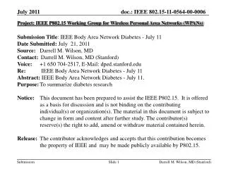
s1 s2 AoA G g LOS W0 sf ToA 1/L 1/l Fig 1: Graphical representation of the CIR as a function of TOA and AOA. Source: 15-06-0195-03-003c
} These first 3 parameters are stored in the data base but not used in the simulation. Is shadowing part of the link budget or should it be included in the simulation? Source: 15-06-0195-03-003c
Start TSV SV TSV or SV Go to slide 19 Go to slide97 Done Done
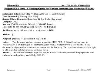
Overview of TSV model Statistical two-path response (LOS desktop model) Fixed impulse response (Other models) Cluster Rician factor (DK) Relative Amplitude ray Rician factor (Dk) S-V model response g: Amplitude of each ray exponentially decays by the order of e -t/g. Time of Arrival Each ray arrives according to the exponential distribution with average value of 1/l Each cluster arrivesaccording to the exponential distribution with average value of 1/L G: Amplitude of each cluster exponentially decays by the order of e-t/G
Definition of TSV model CIR: (Complex impulse response) PLd: Path loss of thefirst impulse response t: time[ns] d(・): Delta function l = cluster number, m= ray number in l-th cluster, L = total number of clusters; Ml = total number of rays in the l-th cluster; Tl = arrival time of the first ray of the l-th cluster; l,m = delay of the m-th ray within the l-th cluster relative to the firs path arrival time, Tl; W0 = Average power of the first ray of the first cluster Yl∝Uniform[0,2p); arrival angle of the first ray within the l-th cluster yl,m = arrival angle of the m-th ray within the l-th cluster relative to the first path arrival angle,Yl Two-path response Arrival rate: Poisson process ANLOS: Constant attenuation for NLOS Two-path parameters (4) S-V parameters (7) Antenna parameters (2) Rician factor (2)
Summary of available TSV channel modelsby MATLAB Measurement and analysis to obtain TSV channel model parameters are finished by NICT. MATLAB code is now available using analyzed parameters.
Channel Model Parameters for TSV model (cont’) ※Antenna gain are calculated by reference antenna model. (Ref. Doc. No. 06-0474)
Function calls in TSV channel model MATLAB code (15-07/0648r0) tg3c_tsv_eval_r7.m (Main script M-file in TSV channel model MATLAB code) tg3c_tsv_params_r4.m tg3c_tsv_ct_r6.m tsv_beta_calc_r5.m tsv_ant_gain_r6.m tsv_laplacernd.m Explained in this documents tsv_poissrnd.m tg3c_sv_cnvrt_ct.m Please see the document “15-06-0468-01-003c” resample.m (built-in function) tg3c_tsv_menu_disp.m (for dialogical parameter input) tg3c_tsv_results_disp.m(to show some figures)
Flowchart of tg3c_tsv_eval_r7.m Red closed line is related to TSV channel model in continuous time Start of TSV model Set channel parameters such as channel model index (cm_num), center frequency (fc0[GHz]),number of channel realizations (num_channels) using function tg3c_tsv_menu_disp.m Call function tg3c_tsv_params_r4.m to load TSV channel model parameters Call function tg3c_tsv_ct_r6.m to generate num_channels sets of amplitude of rays in continuous time (after and/or before antenna gain convolution ) with their TOA and AOA Call function resample.m and then tg3c_tsv_convrt_ct.m to generate num_channels sets of impulse responses (if needed) Save num_channels sets of amplitude, TOA and AOA of rays in continuous time and/or num_channels sets ofdiscrete impulse responses and some of parameters (if needed) Plot the impulse responses, and calculate RMS delay spread and K factor (if needed) done
Summary of tg3c_tsv_eval_r7.m • Main script M-file • This function generates sets of AOA, TOA, and amplitude of rays in continuous time on the basis of TSV model, and also generates and evaluates discrete impulse responses, which are generated using the sets of the AOA, TOA and amplitude of rays in the continuous time. • MATLAB codes distributed in IEEE802.15.4a was modified • This M-file are composed of six sub-functions • tg3c_tsv_param_r4.m • tg3c_tsv_ct_r6.m • tg3c_sv_cnvrt_ct.m • resample.m (built-in function) • tg3c_tsv_menu_disp.m (for dialogical parameter input) • tg3c_tsv_results_disp.m (to show some figures)
function tg3c_tsv_param_r4.m Red closed line is related to TSV channel model in continuous time Start of TSV model Set channel parameters such as channel model index (cm_num), center frequency (fc0[GHz]),number of channel realizations (num_channels) using function tg3c_tsv_menu_disp.m Call function tg3c_tsv_params_r4.m to load TSV channel model parameters Call function tg3c_tsv_ct_r6.m to generate num_channels sets of amplitude of rays in continuous time (after and/or before antenna gain convolution ) with their TOA and AOA Call function resample.m and then tg3c_tsv_convrt_ct.m to generate num_channels sets of impulse responses (if needed) Save num_channels sets of amplitude, TOA and AOA of rays in continuous time and/or num_channels sets ofdiscrete impulse responses and some of parameters (if needed) Plot the impulse responses, and calculate RMS delay spread and K factor (if needed) done Please see the document “15-06-0468-01-003c”
Summary of tg3c_tsv_params_r4.m • This function M-file outputs channel model parameters according to channel model index (cm_num) • Antenna beam-widths described in this function are same as those used for the experiments, but Rx antenna beam-widths can be changed outside this function • Relative power of the LOS component is calculated from carrier frequency (fc [Hz]) and assuming distance (adist [m])
Parameters defined in tg3c_tsv_params_r4.m function [adist, nlos, los_beta_flag, Omega0, smallk, Lmean, Lam, lambda, Gam, ... gamma, std_ln_1, std_ln_2, sigma_fai, L_pl, tx_hpbw, rx_hpbw] = tg3c_tsv_params_r4(cm_num, fc) % Arguments % cm_num channel model number % fc carrier center frequency in GHz % Output parameters % nlos flag of NLOS environment % Lmean number of Average arrival clusters % Lam cluster arrival rate (clusters per nsec) % lambda ray arrival rate (rays per nsec) % Gam cluster decay factor (time constant, nsec) % gamma ray decay factor (time constant, nsec) % std_ln_1 standard deviation of log-normal variable for cluster fading % std_ln_2 standard deviation of log-normal variable for ray fading % sigma_fai cluster angle-of-arrival spread in deg % Parameters added by NICT % adist assuming distance between Tx and Rx in mappded usage model (meter) % los_beta_flag flag used for beta calculation (Renamed from LOS_desktop_flag) % this flag is also used for making LOS extraction for NLOS condition from a LOS condition. % If this value is -1, the LOS component extraction mode is done % Omega0 cluster power level % smallk small Rician factor % L_pl pathloss of the LOS component normalized with that of 1m % tx_hpbw Tx half-power angle in deg % rx_hpbw Rx half-power angle in deg
Example of parameters defined in tg3c_tsv_params_r4.m %************* LOS Residential channel model (UM1) ******************* if cm_num == 11 % Experimental data TX : 360deg, RX : 15deg adist = 5; nlos = 0; los_beta_flag = 0; Omega0 = -88.7; smallk = 4.34; Lmean = 9; Lam = 1/5.24; lambda = 1/0.820; Gam = 4.46; gamma = 6.25; std_ln_1 = 6.28; std_ln_2 = 13.0; sigma_fai = 49.8; tx_hpbw = 360; rx_hpbw = 15; L_pl = -20*log10(4*pi*adist/ramda);
function tg3c_tsv_ct_r6.m Start of TSV model Set channel parameters such as channel model index (cm_num), center frequency (fc0[GHz]),number of channel realizations (num_channels) using function tg3c_tsv_menu_disp.m Call function tg3c_tsv_params_r4.m to load TSV channel model parameters Call function tg3c_tsv_ct_r6.m to generate num_channels sets of amplitude of rays in continuous time (after and/or before antenna gain convolution ) with their TOA and AOA Call function resample.m and then tg3c_tsv_convrt_ct.m to generate num_channels sets of impulse responses (if needed) Save num_channels sets of amplitude, TOA and AOA of rays in continuous time and/or num_channels sets ofdiscrete impulse responses and some of parameters (if needed) Plot the impulse responses, and calculate RMS delay spread and K factor (if needed) done
Summary of tg3c_tsv_ct_r6.m • This function generates sets of AOA, TOA, and power of rays in continuous time on the basis of TSV model • This function consists of four sub-functions • tsv_beta_calc_r5.m • tsv_ant_gain_r6.m • tsv_laplacernd.m • tsv_poissrnd.m
Arguments of tg3c_tsv_ct_r6.m function [beta,h,aoa,t,t0,np,cl_idx] = tg3c_tsv_ct_r6(... nlos, num_channels,... % Channel params adist, fc, los_beta_flg, L_pl,... % T-S-V model params Lam, lambda, Gam, gamma, std_ln_1, std_ln_2, ... % SV model params Lmean, Omega0, smallk, sigma_fai,... tx_hpbw, rx_hpbw, ant_type) % Antenna model params % Arguments: % nlos : Flag of NLOS environment % num_channels : Number of channel realizations % Lam : Cluster arrival rate (clusters per nsec) % lambda : Ray arrival rate (rays per nsec) % Gam : Cluster decay factor (time constant, nsec) % gamma : Ray decay factor (time constant, nsec) % std_ln_1 : Standard deviation of log-normal variable for cluster fading % std_ln_2 : Standard deviation of log-normal variable for ray fading % Lmean : Average number of arrival clusters
Arguments of tg3c_tsv_ct_r6.m (Cont’) % Parameters added for making TG3c channel model % fc : Carrier frequency [GHz] % los_beta_flg : Flag used for beta calculation % L_pl : path loss regarding LOS component % Omega0 : Cluster power level % smallk : Small Rician effect % sigma_fai : Cluster arrival angle spread in deg % tx_hpbw : TX half-power angle in deg % rx_hpbw : RX half-power angle in deg % ant_type : Antenna model used in simulation % 1: Simple Gaussian distribution % 2: Reference antenna model % Output values: % h : Amplitudes of rays in clusters including LOS component in continuous time % t : TOAs of h % t0 : Arrival time of the first ray of the first SV cluster % np : Number of paths in clusters including LOS component % Output values added for making TG3c channel model % beta : Amplitude of the LOS component % aoa : AOAs of rays in clusters including LOS component in continuous time
Modification points in tg3c_tsv_ct_r6.m (1/11) %****************** Initialize and precompute some things ****************** std_L = 1/sqrt(2*Lam); % std dev (nsec) of cluster arrival spacing std_lam = 1/sqrt(2*lambda); % std dev (nsec) of ray arrival spacing %************************** Simulation preparation ************************* h_len = 1000; % there must be a better estimate of # of paths than this ngrow = 1000; % amount to grow data structure if more paths are needed %Output variables beta = zeros(1,num_channels); h = zeros(h_len,num_channels); t = zeros(h_len,num_channels); t0 = zeros(1,num_channels); np = zeros(1,num_channels); aoa = zeros(h_len,num_channels); %added for making TG3c channel model cl_idx = zeros(h_len,num_channels); %added for making TG3c channel model for display Constant value for calculating TOAs of clusters and rays in each cluster Initial number of array for storing results is set to be 1000. This number increases in increments of 1000 if necessary Blue lines are newly added for making TSV MATLAB codes
Modification points in tg3c_tsv_ct_r6.m (2/11) for k = 1:num_channels % loop over number of channels tmp_h = zeros(size(h,1),1); tmp_t = zeros(size(h,1),1); tmp_aoa = zeros(size(h,1),1); %added for making TG3c channel model tmp_clidx = zeros(size(h,1),1); %added for making TG3c channel model %Set the number of generated clusters L = max(1, tsv_poissrnd(Lmean)); % tsv_poisson.m is added for making TG3c channel model %Initialize counter regarding the number of rays in clusters including %LOS component path_ix = 0; Arrays for storing amplitudes, TOAs, and AOAs of rays in one channel realization Counter for counting the number of generated paths Number of clusters are determined according to the Poisson distribution
Modification points in tg3c_tsv_ct_r6.m (3/11) %The following lines are added for making TG3c channel model if nlos==0 % LOS condition expressed by TSV model if los_beta_flg == 1 % Desktop model % Compute LOS component (beta) on the basis of TSV model [beta0] = tg3c_tsv_beta_calc_pre_fin_rev4(fc, adist, tx_hpbw, rx_hpbw, ant_type); beta(k)=beta0; else % The other LOS models % LOS path loss beta(k)=1; end path_ix = path_ix + 1; %path_ix=1; tmp_h(path_ix)=beta(k); tmp_t(path_ix) = 0; tmp_clidx(path_ix) = 1; %LOS component assumed to be a cluster in display tmp_aoa(path_ix) = 0; else % NLOS condition expressed by TSV model if los_beta_flg == -1 % LOS extraction mode beta(k)=0; end end When nlos=0 and LOS_beta_flg =1, beta will be calculated in a function of LOS desktop behavior In the case of all the LOS models except LOS desktop model, b = 1. When nlos =1 and los_beta_flg = -1, LOS extraction mode are applied and beta is set to be 0
Summary of tsv_beta_calc_r5.m • This function computes amplitude of LOS component (beta) on the accordance with the two-path theory of TSV model function [beta] = tsv_beta_calc_r5(fc, muD, tx_hpbw, rx_hpbw, ant_type) % Arguments: % fs : Center carrier frequency % muD : Average distance between TX and RX % tx_hpbw : TX half-power angle in deg % rx_hpbw : RX half-power angle in deg (horizontal and vartical gain are same) % ant_type : Antenna model used in simulation % Output values: % beta : Amplitude of LOS component (beta)
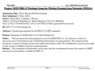
Block diagram of beta calculation in tsv_beta_calc_r5.m D, h1,h2 (in this figure, the heights of Tx and Rx) fluctuates according to the uniform distribution within +-30cm from the average value) Beta can be calculated as below.
How to calculate qt, ft, qr, fr in tsv_beta_calc_r5.m qr jr qt jt D
MATLAB code tsv_beta_calc_r5.m % gamma0 : Reflection coefficient gamma0 = 1; % Assuming angle of incidence is large % these parameters will be discussed D0 = [-0.3 0.3]+muD; % Range of D (m) Ht = [0 0.3]; % Range of Ht (m) Hr = [0 0.3]; % Range of Hr (m) % Determine TX and RX heights by the Monte-carlo method h1 = (Ht(2)-Ht(1))*rand+Ht(1); h2 = (Hr(2)-Hr(1))*rand+Hr(1); % Determine distance between TX and RX by the Monte-carlo method D = (D0(2)-D0(1))*rand+D0(1); % Wave length ramda = 3e8/fc; Determine ranges of D and the heights of Tx and Rx antennas The heights of Tx and Rx antennas vary according to the uniform distribution
MATLAB code tsv_beta_calc_r5.m (Cont’) Calculate qt, ft, qr, frshown in slide X %********** Calculate the reflection point of the reflection path ********** tx_p = i.*h1; rx_p = D+i.*h2; rfl_p = D*h1/(h1+h2); %************ Determinedirection of direct and reflection paths *********** tp = angle([rx_p-tx_p (tx_p-rx_p) rfl_p-tx_p (rfl_p-rx_p)]); tp = tp./pi*180; dr_theta = tp(1); dr_fai = dr_theta; rfl_theta = tp(3); rfl_fai = -rfl_theta; Set the positions of Tx and Rx antennas and the reflection point of radio wave transmitted from Tx in vector Determine angles of departure and arrival of the radio wave in the horizontal axis
MATLAB code tsv_beta_calc_r5.m (Cont’) % TX------------------- % Direct path gt1 = tsv_ant_gain_r6(ant_type, tx_hpbw, dr_theta); % Reflection path gt2 = tsv_ant_gain_r6(ant_type, tx_hpbw, rfl_theta); % RX------------------- % Direct path gr1 = tsv_ant_gain_r6(ant_type, rx_hpbw, dr_fai); % Reflection path gr2 = tsv_ant_gain_r6(ant_type, rx_hpbw, rfl_fai); beta = (muD/D).*abs(gt1.*gr1+gt2.*gr2... .*gamma0.*exp(j.*(2*pi./ramda).*(2.*h1.*h2./D) Determine electric strength of Tx and Rx antennas (in slide X) See the equation expressed in slide X
Summary of tsv_ant_gain_r6.m • This function M-file outputs electric strength according to angle of arrival (AOA). The antenna models contributed in TG3C can be used: • Reference antenna model (IEEE 15-06-0427-04-003c) • Gaussian-distributed antenna model (IEEE 15-06-0195-03-003c) function g = tsv_ant_gain_r6(ant_type, hpbw, fai) % Arguments % ant_type : Antenna model used in simulation % 1: Reference antenna model % 2: Gaussian-distributed antenna model % hpbw : Half-power angle in deg % fai : Angle of arrival in deg % Option % fig_on : Index of figure that shows relative antenna gain % TITLE : figure title % Output value % g : Electric strength (True value)
MATLAB code tsv_ant_gain_r6.m switch ant_type case 1 %Reference antenna model g = zeros(size(fai)); for ii=1:length(fai) theta_ml=2.6*hpbw; G0 = 10*log10((1.6162./sin(hpbw*pi/180/2))^2); if abs(fai(ii))<=theta_ml/2 G = G0 - 3.01 * (2*abs(fai(ii))./hpbw).^2; else G = -0.4111.*log(hpbw)-10.597; end g0=G-G0; g(ii) = 10.^(g0/20); end case 2 %Gaussian-distributed antenna model alfa = 4*log(2)./(hpbw*pi/180).^2; g = sqrt(exp(-alfa.*abs(fai./180*pi).^2)); otherwise error('Antenna model error') end
Modification points of tg3c_tsv_ct_r6.m (4/11) %************************** SV cluster computation ************************* % Determine TOA and AOA of the fisrt SV cluster Tc = (std_L*randn)^2 + (std_L*randn)^2; %added for making TG3c channel model %AOA of clusters is distributed according to the uniform distribution cl_ang_deg = 360*rand-180; if nlos == 1 && los_beta_flg == -1 t0(k) = Tc; end % delta K factor dK = L_pl-Omega0; %added for making TG3c channel model Tc0 = Tc; Determine cluster’s TOA according to the Poisson arrival distribution, which is same as those in 15.3a and 15.4a Calculate AOA of the first cluster. The angle is uniformly distributed from -180 to 180 degree In the case of NLOS condition, the first arrival time of ray is stored, which is used for display Calculate Rician factor (dK)
Modification points of tg3c_tsv_ct_r6.m (5/11) for ncluster = 1:L % relative arrival time of the first ray is set to be 0 in each cluster Tr = 0; %added for making TG3c channel model %fray: flag set to be 1 when it is the first arrival ray fray = 1; Mcluster = std_ln_1*randn; %Pcluster = 10*log10(exp(-1*Tc/Gam))+Mcluster; % total cluster power %added for making TG3c channel model %The first ray of the first cluster is related to delta K factor Pcluster = (-dK-10*(Tc-Tc0)/Gam./log(10))+Mcluster; Process of cluster generation is performed with cluster by cluster TOA of the first ray is set to be 0 in each cluster In the case of only the first ray, flag is set to be 1 The power of a cluster is distributed by the log-normal distribution with variance of std_ln_1 and mean of (dK-10*(Tc-Tc0)/Gam./log(10)). The average power of the first ray in each cluster is dK [dB] because Tc=Tc0
Modification points of tg3c_tsv_ct_r6.m (6/11) Tr_len = 10*gamma; while (Tr < Tr_len), t_val = (Tc+Tr); % TOA of this ray %-------------------------------------------------------------------------------------------------- %The following lines are added for making TG3c channel model % Memo: first ray of the first cluster is set to the mean of the cluster. if fray == 1 % AOA = cluster arrival angle (first ray in each cluster) ray_ang_deg = cl_ang_deg; else % AOA = cluster arrival angle + ray arrival angle % Recalculate if AOA is more than 180 deg or less than -180 deg while 1 % Determine AOA of the ray according to the Laplace distribution in deg ray_ang_deg0 = tsv_laplacernd(sigma_fai); % average is 0 deg if abs(ray_ang_deg0) <= 180 break; end end ray_ang_deg = cl_ang_deg+ray_ang_deg0; end ray_aoa_c = exp(j.*ray_ang_deg./180*pi); aoa_val = angle(ray_aoa_c)/pi*180; The TOA of ray is calculated until Tr is larger than Tr_len(10*gamma), the value of which is same as that written in the 15.4a MATLAB code Calculated TOA of this ray AOA of the first ray is set to the AOA of cluster If the angle is larger than +- 180 degree, the angle is re-generated. The angles of the other ray is Laplace distributed so as that mean values of the rays AOA is the AOA of the cluster. Calculate AOA of the ray in deg
Modification points of tg3c_tsv_ct_r6.m (7/11) Mray = std_ln_2*randn; if fray == 1 %First ray of a cluster %Pray = 10*log10(exp(-Tr/gamma))+Mray; Pray = Mray; %Tr = 0 if small_dk = 0 % Set flag to be 0 after the first-ray's power calculation fray=0; else % Convert the base of small Racian facter small_dk = smallk.*10*log10(exp(1)); Pray = -10*Tr/gamma./log(10)-small_dk+Mray; %Pray=10*log10(exp(-Tr/gamma))-small_dk+Mray; end h_val = 10^((Pcluster+Pray)/20); Pray: power of ray, fray: flag (1:first ray and 0:othres) The power of ray is distributed by the log-normal distribution with variance of std_ln_22 and mean of 10*log10(exp(-Tr/gamma))-small_dk. Amplitude of the ray, fray: flag (1:first ray)
Modification points of tg3c_tsv_ct_r6.m (8/11) % The following lines are the same as that of 15.4a MATLAB code except for some notes % Increment the number of paths path_ix = path_ix + 1; if path_ix > h_len, % grow the output structures to handle more paths as needed tmp_h = [tmp_h; zeros(ngrow,1)]; tmp_t = [tmp_t; zeros(ngrow,1)]; h = [h; zeros(ngrow,num_channels)]; t = [t; zeros(ngrow,num_channels)]; %added for making TG3c channel model tmp_aoa = [tmp_aoa; zeros(ngrow,1)]; tmp_clidx = [tmp_clidx; zeros(ngrow,1)]; aoa = [aoa; zeros(ngrow,num_channels)]; cl_idx = [cl_idx; zeros(ngrow,num_channels)]; Increment the number of rays If prepared arrays are fully occupied, 1000 arrays are added to the old arrays Store the amplitude, TOA, AOA, and cluster index of the ray
Modification points of tg3c_tsv_ct_r6.m (9/11) h_len = h_len + ngrow; end tmp_h(path_ix) = h_val; tmp_t(path_ix) = t_val; tmp_clidx(path_ix) = ncluster+1; %added for making TG3c channel model tmp_aoa(path_ix) = aoa_val; Tr = Tr + (std_lam*randn)^2 + (std_lam*randn)^2; end % Set the TOA and AOA of the next cluster to be generated Tc = Tc + (std_L*randn)^2 + (std_L*randn)^2; cl_ang_deg = 360*rand-180; %added for making TG3c channel model end Set TOA of the next ray Set TOA and AOA of the next cluster
Modification points of g3c_tsv_ct_r6.m (10/11) % The following lines are the same as that of 15.4a MATLAB code except for some notes %********************************* Sorting ********************************* np(k) = path_ix; % Number of rays (or paths) for this realization [sort_tmp_t,sort_ix] = sort(tmp_t(1:np(k))); % sort in ascending time order t(1:np(k),k) = sort_tmp_t; h(1:np(k),k) = tmp_h(sort_ix(1:np(k))); aoa(1:np(k),k) = tmp_aoa(sort_ix(1:np(k))); %added for making TG3c channel model %Attach the generated cluster index to each ray cl_idx(1:np(k),k) = tmp_clidx(sort_ix(1:np(k))); %added for making TG3c channel model
Modification points of tg3c_tsv_ct_r6.m (11/11) %************** Generate continuous complex impulse responses ************** %************** with antenna gain convolution ************** % The following lines are added for making TG3c channel model if op_num == 2 || op_num == 3 tGrh = tsv_ant_gain_r6(ant_type,rx_hpbw, aoa); for ij=1:num_channels tGrh(np(ij)+1:end,ij)=0; end h2 = h.*tGrh; else h2 = []; end Calculate electric strength obtained form AOA of the ray and antenna gain Amplitude or rays are multiplied by the electric strength