1. Introduction

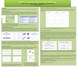
1. Sum 08 1. Introduction Subcanopy advection may explain why ecosystem respiration appears to be underestimated on calm nights. Understanding drainage flows and intermittent mixing at night is only now getting attention in the carbon flux community. 2. Site and instrumentation Harvard Forest (Petersham, MA; 42°30'30'' N; 72°12'28'' W) is a transition mixed deciduous and coniferous forest. Dominant species are red oak (Quercus rubra), red maple (Acer rubrum), black birch (Betula lenta), white pine (Pinus strobus), and eastern hemlock (Tsuga canadensis).. The current study site is focuses at the Little Prospect Hill (LPH) site, where a subcanopy array of 4 2D sonic anemometers where installed around the flux tower at 1.7 m. All sonics point to West. At the tower flux 3 3D sonics were installed at 21, 7, and 1.7 m. The tower flux is measuring almost continuously throughout the year; the subcanopy array measurement campaigns are during the warmer seasons (Table 1). 5. CO2 Budget – integrating subcanopy array data w/ Tower flux data. Nocturnal values of the friction velocity (u*) are larger in spring than in summer, indicating that a leafless canopy produces more wind shear. Figures 6cd show that only during spring is there significant daytime CO2 entry into the domain. There is clear nocturnal CO2 loss due to a persistent downslope drainage flow shown in figure 2. Advective and topographic influences on eddy flux measurementDavid R. Fitzjarrald (1), Ricardo K. Sakai (1), Julian Hadley (2), J. William Munger(2)(1) University at Albany, State University of New York(2) Harvard University Figure 1. a) Current research sites at Harvard Forest. Red borders locate (i) Little Prospect Hill (LPH flux tower and subcanopy array), (ii) the Ant and climate change plot (sodar PA0), (iii) the Environmental monitoring site (EMS flux tower) and d) the EMS canopy tower (PA0 sodar). (Top right insert) Horizontal locations of the subcanopy array and tower setup. The origin is at the LPH tower flux location. Black lines and numbers correspond to the local topography contours (m). Topographic gradient azimuth is 154o, with a slope of 7o (CCW positive). • Table 1: Periods with subcanopy array measurements. • Subcanopy CO2 measurements paused on 01/14/2009 and resumed on 4/15/2009. 3. Subcanopy airflow at the LPH site. (Right and mid-right plots) A remarkable feature of the wind flow within the canopy at LPH is a diurnal motion pattern largely decoupled from the wind aloft. The subcanopy flow is very organized with subcanopy flow follows the local topographic gradient: At night the flow is katabatic (downslope) and during the day it is anabatic (upslope). (Mid left) At the tower flux, azimuth angles show that the flow above (21 m) is disconnect with the subcanopy levels (7 and 1.7 m), but there is still some correlation between 21 and 7 m levels. Between the 7 and 1.7 m levels, there is a good agreement between them in azimuth, but not for the declination. At the 1.7 m the airflow follows the topography gradient axis. (Left): Static stability shows that the highest gradients occurs at the lowest levels, and above and top of the air is more neutral. Figure 4: Median hourly values. Top a) and b) c) flux for summer 2008 and spring and fall 2009. Bottom: a), b), and c) friction velocity. Top d), e) and f)CO2 accumulation . Bottom d), e), and f) Horizontal advection. Sign convection: CO2 leaving the domain: advCO2 >0; CO2 entering the domain: advCO2 <0. 6. Observations of flow over Prospect Hill, HF The two sodars are deployed to examine airflow over the HF topography. Data from the top of EMS tower and the lowest level of data from the nearby sodar (nominally 15 m above canopy) show good agreement during the day, when convective mixing homogenizes the wind profile (Fig. 5a). At night the tower observations fall below 1 m/s on days 200-203 as expected on a calm night with an overlying stable layer; the two agree on subsequent windy nights. The case in Fig. 5a is instructive since synoptic weather changes presented us with a period of westerly winds followed by days with easterly winds. We were surprised to discover that the sodar mean vertical wind values agreed fairly well with those seen by the sonic anemometer at the tower (Fig. 5a, lowest panel), bearing in mind the expected noise in this signal. We see that w < 0 when the EMS tower is on the lee side of Prospect Hill (W wind) and w > 0 when the EMS tower was on the windward side (E wind). We have just begun to analyze sodar data from the Soil Warming Site. This site is not ideal for these measurements. Its choice reflects a balance between adequate housing for our computer and minimal annoyance for the resident scientists and staff at Harvard Forest. In preliminary analysis, however, we have found that data from this site can be suitably filtered to provide useful information (Fig. 5b). For instance, even though there is positive correlation between the horizontal wind velocity for both sodars at EMS and soil warming, their vertical velocities have a negative correlation. This indicates that the sodars can have an acceptable measurement of the airflow over this terrain. Figure 2: (Right) Time series of sonic wind speed components (u, the E-W component, and v, the N-S component) for the Summer 2008 campaign. Ph30m is Campbell Sci. CSAT sonic anemometer at the flux tower, 2D1, 2D2, 2D3, 2D4, and Gill are the ATI 2D and Gill 3D sonic anemometers in the subcanopy layer. (Mid right) Hourly hodographs for spring/summer 08 (a), Fall 08 (b), winter 08/09 (c), and spring 09 (d) for the subcanopy and at the top of the tower (on the bottom right side) sonic anemometers. Numbers in the hodographs are the local time hour. Black lines are the local elevation contours relative to the tower elevation. (Mid Left) Scatter plots of airflow angles among 3D sonics at the flux tower (21 m, 7m, and 1.7m). Blue “+” represents daytime values, black “o” represents nighttime values. Azimuth of the streamflow (Azim) is defined as the angle of the horizontal wind vector with the geographic north. Declination of streamflow is defined as the angle of the vertical wind with the geographic horizon. (Left) Top – Time series of air temperature gradients at tower flux. Bottom: Mean hourly values of the air temperature gradients. 4. Subcanopy CO2 distribution. Marked spatial differences on CO2 concentrations are only observed with leaf coverage.- When the canopy starts to leaf out; CO2 deviations become significant (Fig. 3 b and d). Higher locations (#3 and #4) present the lowest concentration, principally during nighttime. Slope of the CO2 surfaces is about parallel to the streamline, with the declination of the streamline being smaller than the slope of the topography. Fig. 5.(a) Winds at the PA0 sodar (black) lowest reporting level and the EMS tower (blue) at the EMS site days 199-207, 2008. Top: wind speed (m/s); middle: wind direction (degrees) ; bottom: vertical velocity (m/s). Solid lines are smoothed versions of the half-hourly data. (b) 2009 DOY 137-48 (UT) half-hourly time series comparison of (top) wind direction; (middle) wind speed and (bottom) mean vertical wind speed between the EMS site PA0 sodar (red, triangles) and the soil warming site PA1 sodar (black, squares). Fal 08 Sum 08 6 .Conclusion The subcanopy array shows a strong advection within the canopy that is decoupled with the air aloft at nighttime. Only significant horizontal CO2 gradients were observed during spring and summer at the forest floor. These observations show that the canopy storage is less important than either the flux through canopy top or the advection on the sides of the domain. (Note that we performed no ‘u* filtering’ for the CO2 flux.). At night, horizontal advection is about the same magnitude as the observed vertical flux, occasionally exceeding the above-canopy average CO2 flux. We found good agreement among both sodars and tower flux measurements. Nowadays, the task is to test the ‘flow over hill’ hypothesis in which Bernoulli effects associated with flow over hills strongly affect subcanopy motions, possibly altering horizontal CO2 advection. We aim to categorize above-canopy flows by direction and intensity, compare flow upwind and downwind of the major topographic features, and determine the extent to which subcanopy flows are altered. The final step is to document if any effects are sufficient to modify the role of horizontal advection on the subcanopy CO2 budget. 7. Acknowledgements: This work has been fully supported by DOE, Project ID 0013717. Win09 Spr09 Figure 4: Angles for the air flow (top) and CO2 surface at 1.7 m. Airflow angles were estimated using the 1.7 m 3D sonic, and the CO2 surface angle were estimated calculating the CO2 spatial concentration gradients at 1.7 m. Vertical solid lines correspond to the azimuth of the topographic gradient (154o), and the horizontal solid line the slope of the local topography (7.4 o). Blue “+” represents daytime values, black “o” represents nighttime values. Figure 3. Time series of CO2 concentration and perturbation at the subcanopy surface array for summer 2008 (a) and spring 2009); (b). Locations #1, #2, #3, #4, and #5 are related to 2D1, 2D2, 2D3, 2D4, and, Gill respectively. (c) and (d) correspond to the mean hourly values of the CO2 concentration and CO2 concentration deviations for summer 2008, and spring 2009 respectively.