The Disappearance of the Aral Sea: Causes and Consequences (1973-2000)
460 likes | 581 Views
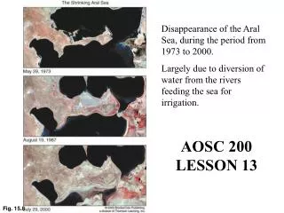
The Aral Sea, once one of the world's largest inland bodies of water, has drastically shrunk from 1973 to 2000 primarily due to the diversion of rivers for irrigation, particularly for cotton farming in the Soviet Union. This environmental tragedy led to increased salinity, decimated local fishing industries, and transformed the region into an "Asian Dust Bowl." Climate changes have also contributed to altered weather patterns, emphasizing the far-reaching impact of human decision-making on ecosystems.

The Disappearance of the Aral Sea: Causes and Consequences (1973-2000)
E N D
Presentation Transcript
Disappearance of the Aral Sea, during the period from 1973 to 2000. Largely due to diversion of water from the rivers feeding the sea for irrigation. AOSC 200 LESSON 13 Fig. 15.8
Human Influences on Climate • Greenhouse effect • Feedbacks • Northward movement of the jet streams • Changing Land Surfaces • Heat Islands • Consequences of Greenhouse Effect
CLIMATE FEEDBACK MECHANISMS • POSITIVE AND NEGATIVE FEEDBACKS • WATER VAPOR - POSITIVE • CLOUDS - POSITIVE AND NEGATIVE - MAINLY NEGATIVE
Positions of the jet streams Fig. 7-27, p. 191
Jet Streams on March 11, 1990Sub-tropical = Blue, Polar = Red
Relation between jet stream and high and low pressure systems Fig. 8-30, p. 231
Frontal Movement and Climate Change • Increasing evidence that the Polar and Sub-tropical jet streams in the Northern Hemisphere are moving northward. • This implies that the weather patterns associated with the jets (fronts) are also moving northward • As the sub-tropical jet moves northward so do the high pressure systems associated with this jet. • Expect drier summers • Could increase in greenhouse forcing in the tropics lead to a stronger Hadley cell circulation, and hence to a movement of the jet?
Disappearance of the Aral Sea, during the period from 1973 to 2000. Largely due to diversion of water from the rivers feeding the sea for irrigation. Fig. 15.8
Aral Sea • Government of the Soviet Union diverted waters feeding this inland lake to provide water for the growing of cotton. • Aral Sea began shrinking rapidly • Climate has also changed in the region • Asian ‘Dust Bowl’ • Increased salinity destroyed fishing industry
Roadways and buildings reduce evapor-transpiration and absorb more solar radiation than the surrounding rural regions. Fig. 15.9
THE CLIMATE OF CITIES • URBAN HEAT ISLAND • TEMPERATURES ARE GENERALLY HIGHER THAN IN RURAL AREAS, CREATING AN 'ISLAND' OF WARMER AIR. • CITIES ARE GENERALLY CLOUDIER, FOGGIER, WARMER, WETTER • WHY? • ROCK-LIKE MATERIALS OF CITY HAVE HIGH THERMAL CAPACITY • IMPERVIOUS SURFACES REMOVE PRECIPITATION QUICKLY • LARGE SOURCES OF HEAT • ATMOSPHERIC POLLUTION TRAPS RADIATION • TALL BUILDINGS ALTER THE AIR FLOW • INCREASED PRECIPITATION • THERMALLY INDUCED UPWARD MOTIONS
CONSEQUENCES OF GREENHOUSE WARMING • .WATER RESOURCES AND AGRICULTURE - CHANGES IN PRECIPITATION PATTERNS - LENGTH OF GROWING SEASON • .SEA LEVEL RISE - .MELTING OF GLACIERS PLUS THE THERMAL EXPANSION OF THE OCEANS - HAS RISEN 10-25 CM OVER PAST CENTURY • .NEW WEATHER PATTERNS - HIGHER FREQUENCY AND GREATER INTENSITY OF HURRICANES BECAUSE OF WARMER SEA SURFACE TEMPERATURES. • SHIFTS IN PATHS OF CYCLONIC STORMS - PRECIPITATION PATTERNS. • .SHIFTS OF OCCURRENCES OF TORNADOES. • .MORE INTENSE HEAT WAVES AND DROUGHTS IN SOME REGIONS AND LESS IN OTHERS.
Air Pollution William Shakespeare 1564-1616, from his play ‘Hamlet’
History of Air Pollution • Air pollution is not a new problem • In England, wood for burning became scarce, and the populace resorted to burning coal which had a high sulfur content. The by-products were soot (carbon particles) and sulfur dioxide. • John Evelyn in 1661 wrote about the notorious London pea-soup fog. These occur in the fall when the Thames is warm but the ground is cold. The natural fog this produces is enhanced by the extra soot particles, and the sulfur dioxide reacts in the water droplets to produce sulfuric acid.
SMOG • Word coined by Dr. Harold Des Veaux, a London physician in 1903. • SMOKE + FOG = SMOG • He meant London smog – sulfurous fumes from coal burning + large water droplets formed around smoke particles (soot) • 1952 – Killer smog – 4000 deaths. Another episode in 1956 led to 1000 deaths. • Similar events have also occurred in the US. • Large industrial cities such as St.Louis and Pittsburg also suffered from ‘London’ smog, as the use of coal increased.
PHOTOCHEMICAL SMOG • In 1940 vegetable crop damage began to be seen in the Los Angeles basin. Pine trees began to lose their needles. • Haagen-Smit and colleagues at the University of California, Riverside studied this effect using smog chambers - large plastic tents into which pollutants could be injected and their reactions investigated. • They showed that the effect was due to ozone in the atmosphere. • The ozone was produced by a series of reactions involving the oxides of nitrogen and organic compounds (e.g. gasoline), both of which are emitted by automobiles. • It is this form of smog that gives the pollution seen in the Baltimore/Washington corridor.
Sources and Types of Air Pollutants • can be grouped into two categories: primary and secondary. • Primary pollutants are emitted directly from identifiable sources. They pollute the air immediately upon being emitted. • Secondary pollutants are produced in the atmosphere when certain chemical reactions take place among primary pollutants. • Sources. Two types of sources are identified fixed sources and mobile sources.
Composition of the Earth’s Troposphere H2 PM O2 CH4 N2 CO N2O O3 ←SO2, NO2, CFC’s, etc Ar CO2 Inert gases
PM is made up of suspended particles of either solid or liquid pollutants. PM is grouped by size: under 10 microns is called PM10, under 2.5 microns is called PM2.5. PM causes increased mortality and morbidity. Examples of PM include diesel soot, acids, dust, sulfates, nitrates, and organics. Fine Particles or Particulate Matter (PM)
Schematic of ozone production from a Volatile Organic Compound (VOC)
SMOG • NEEDS • Hydrocarbons and nitrogen oxides • Strong sunlight to start reactions • Warm temperatures to maintain reactions – the higher the temperature the faster the rate. • Peak ozone will be when temperature is highest – in the afternoon.
Daily Ozone Cycle Ozone production follows a daily cycle with maximum concentrations typically observed in the late afternoon. This cycle is a signature of the dynamic processes of atmospheric air pollution Ozone Concentration Sunrise Sunset Time of day
High Pollution days • The figure illustrates one of the problems in the abatement of pollution. The ozone concentration is used as the standard, and yet one can reduce the nitrogen oxides by a significant fraction and see no change, or even an increase in the ozone level. • Most of the pollution is emitted in the cities, which typically puts the atmosphere at the right of the figure. As the pollutants move away from the city center their concentration gets smaller, and the atmosphere is moved toward the left, and the ozone increases. • Hence the suburbs can see more ozone than the cities.