Falkner-Skan Solutions
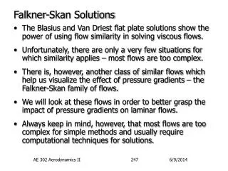
Falkner-Skan Solutions. The Blasius and Van Driest flat plate solutions show the power of using flow similarity in solving viscous flows. Unfortunately, there are only a very few situations for which similarity applies – most flows are too complex.

Falkner-Skan Solutions
E N D
Presentation Transcript
Falkner-Skan Solutions • The Blasius and Van Driest flat plate solutions show the power of using flow similarity in solving viscous flows. • Unfortunately, there are only a very few situations for which similarity applies – most flows are too complex. • There is, however, another class of similar flows which help us visualize the effect of pressure gradients – the Falkner-Skan family of flows. • We will look at these flows in order to better grasp the impact of pressure gradients on laminar flows. • Always keep in mind, however, that most flows are too complex for simple methods and usually require computational techniques for solutions. AE 302 Aerodynamics II
Falkner-Skan Solutions (2) • First, lets start with the B.L. equations including the pressure term we dropped for Blasius solution. • The pressure return we will eliminate by using Euler’s equation in the freestream: • Based upon what we learned from the Blasius solution we will assume that the horizontal velocity and y coordinate can be represented by: AE 302 Aerodynamics II
Falkner-Skan Solutions (3) • In the Blasius solution we used the stream function to automatically satisfy flow continuity. • This time take a different approach and use continuity to eliminate the vertical velocity from our equation. • Were the boundary conditions have been used to evaluate the integral at y=0: • The remaining momentum equation is now: AE 302 Aerodynamics II
Falkner-Skan Solutions (4) • In expanding this this equation, we need to expand the derivative in terms of the transformed variables: • Realize that that the freestream velocity is no longer a constant but varies with x (or ) and that we do not yet know the form of g: AE 302 Aerodynamics II
Falkner-Skan Solution (5) • Putting this into the momentum equation gives: • Or, after rearranging: • In order to have similarity, all dependence upon x must disappear from the above expression – or rather, the two multipliers above must be equal to constants: AE 302 Aerodynamics II
Falkner-Skan Solution (6) • Falner and Skan found that this could be achieved if the transform and velocity were expressed by power laws: • The also choose the constants C and K to be compatible with Blasius for the case of zero pressure gradient, m=0: • In this case: • And the governing equation becomes: AE 302 Aerodynamics II
x x Wedge Flow 0< <2 0<m< Expansion Corner -2< <0 -1/2<m<0 Falkner-Skan Wedge Flows • It is natural to ask what exactly are the flows described by the power law type velocity variation: • It turns out that this equation describes the flow over wedges. • Note the first case is a decelerating velocity, i.e. adverse pressure gradient, while the second case is accelerating and thus favorable. AE 302 Aerodynamics II
Falkner-Skan Wedge Flows (2) • The wedge flow case has some usefulness. • The expansion corner, by contrast, is not realistic since the B.L does not begin until AFTER the corner. • However, both cases provide tremendous insight into the behavior of laminar B.L.’s under a pressure gradient. • The solutions for Falkner-Skan flow for b from near 2 to -0.1988 are shown on the following page. • The limit of b 2 (m) is for an extremely rapidly accelerating flow. • Also, while the shape has a similar shape, the B.L. thickness is decreasing as velocity increases. AE 302 Aerodynamics II
Falkner-Skan Wedge Flows (3) AE 302 Aerodynamics II
Falkner-Skan Wedge Flows (4) • The other limit, b -0.1988 (m-0.0904) is the point of incipient separation. • At this point, the velocity gradient at the wall is zero – i.e. there is no wall shear stress. • Beyond this point there is no possible solution to the equation – which tells us that separated flows are not similar in nature. • This makes sense since separated flows must have a separation point – and thus cannot have the same shape before and after separation. AE 302 Aerodynamics II
Momentum Integral Equation • Before leaving laminar flow and moving on to turbulence, there is one other special equation of note. • Begin with the incompressible momentum equation with the integral continuity equation replacing the vertical velocity: • No consider if we integrated this momentum equation across the B.L. – from the wall to the freestream: AE 302 Aerodynamics II
Momentum Integral Equation (2) • The right hand side term integrates directly to give: • Also, the middle term on the left hand side can be integrated by parts: • With these two expressions, our integral equation becomes: AE 302 Aerodynamics II
Momentum Integral Equation (3) • The new middle term can be expanded: • So that the integral equation can be rewritten as: • Now compare this with the definitions of displacement and momentum thickness: AE 302 Aerodynamics II
Momentum Integral Equation (4) • From the comparison, we see that our final equation can be rewritten in terms of * and as: • This is the Momentum Integral Equation, an simplified form of the incompressible Boundary Layer Equations. • Because we integrated across the B.L., this equation does not involve the details of the B.L. shape. • In fact, solutions to this equation can be thought of as satisfy the original B.L. equations on average rather than exactly. AE 302 Aerodynamics II
Pohlhausen Solution • To solve the Momentum Integral Equation, we need to relate all the variables, V, *, and w, by assuming a shape to the B.L. • A popular approach was proposed by Pohlhausen who used a quadratic equation for his family of B.L.’s in the form: • Which satisfies the boundary conditions: AE 302 Aerodynamics II
Pohlhausen Solution (2) • The factor , determines the B.L. profile shape and depends upon the velocity gradient in the freestream: AE 302 Aerodynamics II
Pohlhausen Solution (3) • The combination of the Momentum Integral Equation with the assumed shape results in an ODE in x. • This equation can be numerically marched in the x direction starting with suitable initial conditions. • The results, while approximate, yields pretty accurate solutions for the B.L. thicknesses and shear stress – for considerably less effort than solving the original PDE’s. • For a flat plate, the results are: AE 302 Aerodynamics II
Pohlhausen Solution (4) • Another important observation about Pohlhausen’s solution, without solving it, is about separation. • The family of B.L. shapes shows that separation occurs for ~-12. • But: • Thus, we see that we must have a negative velocity gradient (positive pressure gradient) for separation. • As important, we see that “young” B.L.’s, where is small, can withstand higher gradients before separating. • “Old” B.L.’s which are thicker, will separate earlier. AE 302 Aerodynamics II