Download
1 / 61
620 likes | 896 Views
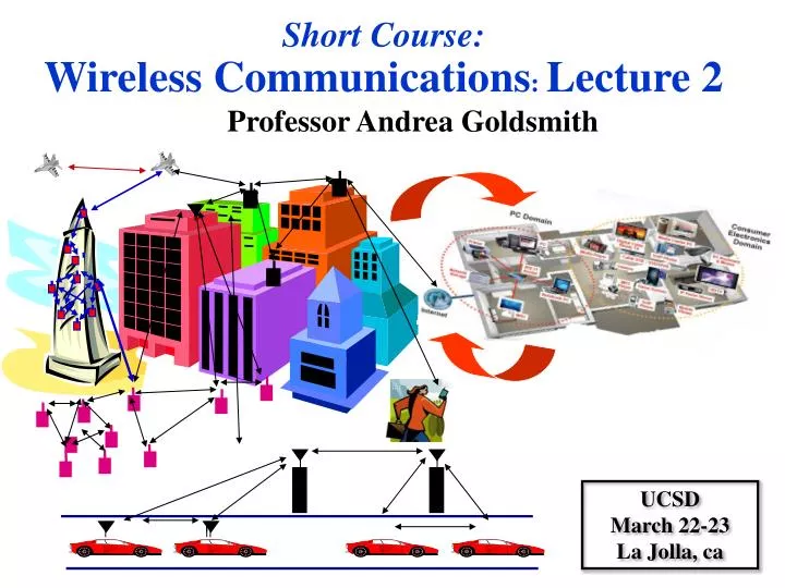
Short Course: Wireless Communications : Lecture 2. Professor Andrea Goldsmith. UCSD March 22-23 La Jolla, ca. Course Outline. Overview of Wireless Communications Path Loss, Shadowing, and WB/NB Fading Capacity of Wireless Channels Digital Modulation and its Performance

E N D
Short Course: Wireless Communications: Lecture 2 Professor Andrea Goldsmith UCSD March 22-23 La Jolla, ca
Course Outline • Overview of Wireless Communications • Path Loss, Shadowing, and WB/NB Fading • Capacity of Wireless Channels • Digital Modulation and its Performance • Adaptive Modulation • Diversity • MIMO Systems • Multicarrier Modulation • Spread Spectrum • Multiuser Communications & Wireless Networks • Future Wireless Systems Lecture 1 Lecture 2
Future Wireless Networks Ubiquitous Communication Among People and Devices Wireless Internet access Nth generation Cellular Wireless Ad Hoc Networks Sensor Networks Wireless Entertainment Smart Homes/Spaces Automated Highways All this and more… • Hard Delay/Energy Constraints • Hard Rate Requirements
d Pr/Pt d=vt Signal Propagation • Path Loss • Shadowing • Multipath
Statistical Multipath Model • Random # of multipath components, each with varying amplitude, phase, doppler, and delay • Narrowband channel • Signal amplitude varies randomly (complex Gaussian). • 2nd order statistics (Bessel function), Fade duration, etc. • Wideband channel • Characterized by channel scattering function (Bc,Bd)
Capacity of Flat Fading Channels • Three cases • Fading statistics known • Fade value known at receiver • Fade value known at receiver and transmitter • Optimal Adaptation • Vary rate and power relative to channel • Optimal power adaptation is water-filling • Exceeds AWGN channel capacity at low SNRs • Suboptimal techniques come close to capacity
Modulation Considerations • Want high rates, high spectral efficiency, high power efficiency, robust to channel, cheap. • Linear Modulation (MPAM,MPSK,MQAM) • Information encoded in amplitude/phase • More spectrally efficient than nonlinear • Easier to adapt. • Issues: differential encoding, pulse shaping, bit mapping. • Nonlinear modulation (FSK) • Information encoded in frequency • More robust to channel and amplifier nonlinearities
dmin Linear Modulation in AWGN • ML detection induces decision regions • Example: 8PSK • Ps depends on • # of nearest neighbors • Minimum distance dmin (depends on gs) • Approximate expression
Ps Ts Linear Modulation in Fading • In fading gsand therefore Psrandom • Metrics: outage, average Ps , combined outage and average. Ts Ps Outage Ps(target)
Tm ISI Effects • Delay spread exceeding a symbol time causes ISI (self interference). • ISI leads to irreducible error floor • Increasing signal power increases ISI power • Without compensation, requires Ts>>Tm • Severe constraint on data rate (Rs<<Bc) 1 2 3 4 5 0 Ts
Main Takeaway • Narrowband wireless channel characterized by random flat-fading (Bu<<Bc) • Wideband wireless channel characterized by random frequency-selective fading (ISI) • Need to combat flat and frequency-selective fading • Focus of this section of short course
Course Outline • Overview of Wireless Communications • Path Loss, Shadowing, and Fading Models • Capacity of Wireless Channels • Digital Modulation and its Performance • Adaptive Modulation • Diversity • MIMO Systems • Multicarrier Modulation • Spread Spectrum • Multiuser Communications & Wireless Networks • Future Wireless Systems
Adaptive Modulation • Change modulation relative to fading • Parameters to adapt: • Constellation size • Transmit power • Instantaneous BER • Symbol time • Coding rate/scheme • Optimization criterion: • Maximize throughput • Minimize average power • Minimize average BER Only 1-2 degrees of freedom needed for good performance
One of the M(g) Points log2 M(g) Bits To Channel M(g)-QAM Modulator Power: P(g) Point Selector Uncoded Data Bits Delay g(t) g(t) 16-QAM 4-QAM BSPK Variable-Rate Variable-Power MQAM Goal: Optimize P(g) and M(g) to maximize R=Elog[M(g)]
Optimization Formulation • Adaptive MQAM: Rate for fixed BER • Rate and Power Optimization Same maximization as for capacity, except for K=-1.5/ln(5BER).
gk g Optimal Adaptive Scheme • Power Adaptation • Spectral Efficiency g Equals capacity with effective power loss K=-1.5/ln(5BER).
K2 K1 K=-1.5/ln(5BER) Spectral Efficiency Can reduce gap by superimposing a trellis code
Constellation Restriction • Restrict MD(g) to {M0=0,…,MN}. • Let M(g)=g/gK*, where gK* is later optimized. • Set MD(g) to maxj Mj: Mj M(g). • Region boundaries are gj=MjgK*, j=0,…,N • Power control maintains target BER M3 M(g)=g/gK* MD(g) M3 M2 M2 M1 M1 Outage 0 g0 g1=M1gK* g2 g3 g
Power Adaptation and Average Rate • Power adaptation: • Fixed BER within each region • Es/N0=(Mj-1)/K • Channel inversion within a region • Requires power increase when increasing M(g) • Average Rate
Efficiency in Rayleigh Fading Spectral Efficiency (bps/Hz) Average SNR (dB)
Constellation Restriction M3 M(g)=g/gK* MD(g) M3 M2 M2 M1 M1 Outage 0 g0 g1=M1gK* g2 g3 g • Power adaptation: • Average rate:
Efficiency in Rayleigh Fading Spectral Efficiency (bps/Hz) Average SNR (dB)
Practical Constraints • Constellation updates: fade region duration • Error floor from estimation error • Estimation error at RX can cause error in absence of noise (e.g. for MQAM) • Estimation error at TX causes mismatch of adaptive power and rate to actual channel • Error floor from delay: let r(t,t)=g(t-t)/g(t). • Feedback delay causes mismatch of adaptive power and rate to actual channel
Detailed Formulas ^ • Error floor from estimation error () • Joint distribution p(,) depends on estimation: hard to obtain. For PSAM the envelope is bi-variate Rayleigh • Error floor from delay: let =g[i]/g[i-id]. • p(|) known for Nakagami fading ^
Main Points • Adaptive modulation leverages fast fading to improve performance (throughput, BER, etc.) • Adaptive MQAM uses capacity-achieving power and rate adaptation, with power penalty K. • Comes within 5-6 dB of capacity • Discretizing the constellation size results in negligible performance loss. • Constellations cannot be updated faster than 10s to 100s of symbol times: OK for most dopplers.
Course Outline • Overview of Wireless Communications • Path Loss, Shadowing, and WB/NB Fading • Capacity of Wireless Channels • Digital Modulation and its Performance • Adaptive Modulation • Diversity • MIMO Systems • Multicarrier Modulation • Spread Spectrum • Multiuser Communications & Wireless Networks • Future Wireless Systems
Tb Introduction to Diversity • Basic Idea • Send same bits over independent fading paths • Independent fading paths obtained by time, space, frequency, or polarization diversity • Combine paths to mitigate fading effects t Multiple paths unlikely to fade simultaneously
Combining Techniques • Selection Combining • Fading path with highest gain used • Maximal Ratio Combining • All paths cophased and summed with optimal weighting to maximize combiner output SNR • Equal Gain Combining • All paths cophased and summed with equal weighting • Array/Diversity gain • Array gain is from noise averaging (AWGN and fading) • Diversity gain is change in BER slope (fading)
Selection Combining Analysis and Performance • Selection Combining (SC) • Combiner SNR is the maximum of the branch SNRs. • CDF easy to obtain, pdf found by differentiating. • Diminishing returns with number of antennas. • Can get up to about 20 dB of gain. Outage Probability
MRC and its Performance • With MRC, gS=gifor branch SNRsgi • Optimal technique to maximize output SNR • Yields 20-40 dB performance gains • Distribution of gS hard to obtain • Standard average BER calculation Recall • Integral hard to obtain in closed form and often diverges
MGF Approach • Use alternate form of Q function • Define the MGF of gi as • Laplace transform of distribution • Often simple closed form expressions • Rearranging order of integration, we get g depends on modulation (a,b)
EGC and Transmit Diversity • EGQ simpler than MRC • Harder to analyze • Performance about 1 dB worse than MRC • Transmit diversity • With channel knowledge, similar to receiver diversity, same array/diversity gain • Without channel knowledge, can obtain diversity gain through Alamouti scheme: works over 2 consecutive symbols
Main Points • Diversity typically entails some penalty in terms of rate, bandwidth, complexity, or size. • Techniques trade complexity for performance. • MRC yields 20-40 dB gain, SC around 20 dB. • Analysis of MRC simplified using MGF approach • EGC easier to implement than MRC: hard to analyze. • Performance about 1 dB worse than MRC • Transmit diversity can obtain diversity gain even without channel information at transmitter.
Course Outline • Overview of Wireless Communications • Path Loss, Shadowing, and Fading Models • Capacity of Wireless Channels • Digital Modulation and its Performance • Adaptive Modulation • Diversity • MIMO Systems • Multicarrier Modulation • Spread Spectrum • Multiuser Communications & Wireless Networks • Future Wireless Systems
MIMO Systems and their Decomposition • MIMO (multiple-input multiple-output) systems have multiple transmit and receive antennas • Decompose channel through transmit precoding (x=Vx) and receiver shaping (y=UHy) • Leads to RHmin(Mt,Mr) independent channels with gain si (ith singular value of H) and AWGN • Independent channels lead to simple capacity analysis and modulation/demodulation design ~ ~ ~ y=S x+n y=Hx+n H=USVH ~ ~ ~ yi=six+ni ~ ~
Capacity of MIMO Systems • Depends on what is known at TX and RX and if channel is static or fading • For static channel with perfect CSI at TX and RX, power water-filling over space is optimal: • In fading waterfill over space (based on short-term power constraint) or space-time (long-term constraint) • Without transmitter channel knowledge, capacity metric is based on an outage probability • Pout is the probability that the channel capacity given the channel realization is below the transmission rate.
Beamforming • Scalar codes with transmit precoding y=uHHvx+uHn • Transforms system into a SISO system with diversity. • Array and diversity gain • Greatly simplifies encoding and decoding. • Channel indicates the best direction to beamform • Need “sufficient” knowledge for optimality of beamforming
Optimality of Beamforming Covariance Information Mean Information
Error Prone Low Pe Diversity vs. Multiplexing • Use antennas for multiplexing or diversity • Diversity/Multiplexing tradeoffs (Zheng/Tse) Best use depends on the application
ST Code High Rate High-Rate Quantizer Decoder Error Prone ST Code High Diversity Low-Rate Quantizer Decoder Low Pe How should antennas be used? • Use antennas for multiplexing: • Use antennas for diversity Depends on end-to-end metric: Solve by optimizing app. metric
MIMO Receiver Design • Optimal Receiver: • Maximum likelihood: finds input symbol most likely to have resulted in received vector • Exponentially complex # of streams and constellation size • Decision-Feedback receiver • Uses triangular decomposition of channel matrix • Allows sequential detection of symbol at each received antenna, subtracting out previously detected symbols • Sphere Decoder: • Only considers possibilities within a sphere of received symbol. • Space-Time Processing: Encode/decode over time & space
Other MIMO Design Issues • Space-time coding: • Map symbols to both space and time via space-time block and convolutional codes. • For OFDM systems, codes are also mapped over frequency tones. • Adaptive techniques: • Fast and accurate channel estimation • Adapt the use of transmit/receive antennas • Adapting modulation and coding. • Limited feedback: • Partial CSI introduces interference in parallel decomp: can use interference cancellation at RX • TX codebook design for quantized channel
Main Points • MIMO systems exploit multiple antennas at both TX and RX for capacity and/or diversity gain • With TX and RX channel knowledge, channel decomposes into independent channels • Linear capacity increase with number of TX/RX antennas • With TX/RX channel knowledge, capacity vs. outage is the capacity metric • Beamforming provides diversity gain in direction of dominent channel eigenvectors • Fundamental tradeoff between capacity increase and diversity gain: optimization depends on application
Main Points • MIMO RX design trades complexity for performance • ML detector optimal; exponentially complex • DF receivers prone to error propagation • Sphere decoders allow performance tradeoff via radius • Space-time processing (i.e. coding) used in most systems • Adaptation requires fast/accurate channel estimation • Limited feedback introduces interference between streams: requires codebook design
ISI Countermeasures • Equalization • Signal processing at receiver to eliminate ISI, must balance ISI removal with noise enhancement • Can be very complex at high data rates, and performs poorly in fast-changing channels • Not that common in state-of-the-art wireless systems • Multicarrier Modulation • Break data stream into lower-rate substreams modulated onto narrowband flat-fading subchannels • Spread spectrum • Superimpose a fast (wideband) spreading sequence on top of data sequence, allows resolution for combining or attenuation of multipath components.
Course Outline • Overview of Wireless Communications • Path Loss, Shadowing, and Fading Models • Capacity of Wireless Channels • Digital Modulation and its Performance • Adaptive Modulation • Diversity • MIMO Systems • Multicarrier Modulation • Spread Spectrum • Multiuser Communications & Wireless Networks • Future Wireless Systems
S cos(2pf0t) cos(2pfNt) x x Multicarrier Modulation R/N bps • Breaks data into N substreams • Substream modulated onto separate carriers • Substream bandwidth is B/N for B total bandwidth • B/N<Bc implies flat fading on each subcarrier (no ISI) QAM Modulator R bps Serial To Parallel Converter R/N bps QAM Modulator
Overlapping Substreams • Can have completely separate subchannels • Required passband bandwidth is B. • OFDM overlaps substreams • Substreams (symbol time TN) separated in RX • Minimum substream separation is BN/(1+b). • Total required bandwidth is B/2 (for TN=1/BN) B/N fN-1 f0
Fading Across Subcarriers • Leads to different BERS • Compensation techniques • Frequency equalization (noise enhancement) • Precoding • Coding across subcarriers • Adaptive loading (power and rate)