Download
1 / 41
410 likes | 509 Views
Flavour physics after the first run of the LHC. Diego Martinez Santos (NIKHEF, VU Amsterdam and CERN). On behalf of the LHCb Collaboration Including also ATLAS and CMS results. Introduction.

E N D
Flavour physics after the first run of the LHC Diego Martinez Santos (NIKHEF, VU Amsterdam and CERN) On behalf of the LHCb Collaboration Including also ATLAS and CMS results BSM after the first run of the LHC. Galileo Galilei Institute. Firenze, 10/07/2013
Introduction • The SM is very successful in accurately describing accelerator data, yet it is known to be an incomplete theory (gravity, DM, etc…) • Several alternatives/extension exist (SUSY, compositeness, ED’s … ) which could be a better approach to nature • Need (new) experimental data to: • Break SM (if possible) at accelerators • Constrain BSM parameters, rule out models inconsistent with data … • Two main approaches at LHC • Direct search of new particles ATLAS/CMS • Indirect search LHCb • Access to BSM physics through its effect in B,D,K,τ decays • This approach has been very successful in many cases: top quark or Z0 were inferred from indirect effects many years before direct observation BSM after the first run of the LHC. Galileo Galilei Institute. Firenze, 2013
A nice parallelism ? The Ptolemaic model was very successful on precisely describe all astronomic data for many years. (very much like SM) Alternate (i.e. heliocentric) models existed since Aristarchos (c.III BC), but they predicted unobserved phenomena like parallax -not observed till c.XIX-, which could only fit if one puts the distance of the stars at a very large scale. (very much like BSM) In c.XVII, Galileo points the first telescope to the sky and observes a series of phenomena that contradicted Ptolemaic model, and favoured heliocentric theories…. (very much like LHC ??) BSM after the first run of the LHC. Galileo Galilei Institute. Firenze, 2013
Flavour physics results from LHCb • Very rare decays • Light flavoured mesons decaying into dimuons: • Bs→ µµ, Bd→ µµ, D0→ µµ, KS→ µµ • Other very rare decays • Results in CPV • Electroweak phase • First observation of CPV in Bs decays • CPV in charm • The rare decay Bd→ K* µµ • Nice flavour topics not covered here: radiative decays, measurement of CKM angle γ BSM after the first run of the LHC. Galileo Galilei Institute. Firenze, 2013
Flavour physics results from LHCb • Very rare decays • Light flavoured mesons decaying into dimuons: • Bs→ µµ, Bd→ µµ, D0→ µµ, KS→ µµ • Other very rare decays • Results in CPV • Electroweak phase • First observation of CPV in Bs decays • CPV in charm • The rare decay Bd→ K* µµ • I will also cover some ATLAS and CMS results BSM after the first run of the LHC. Galileo Galilei Institute. Firenze, 2013
VERY RARE DECAYS BSM after the first run of the LHC. Galileo Galilei Institute. Firenze, 2013
Bs(d) → µµ These decays are very supressed in SM arXiv:1208.0934. BR(Bs→ µµ) = (3.54 ± 0.30)x10-9 BR(Bd→ µµ) = (1.07 ± 0.10)x10-10 (time averaged) … but can be modified by NP. Here you have a rough table of what would imply each potential result (note tha the arrow goes only in one direction) BSM after the first run of the LHC. Galileo Galilei Institute. Firenze, 2013
Bs(d) → µµ (LHCb analysis strategy) arXiv:1211.2674 PhysRevLett.110.021801 • I) Selection cuts in order to reduce the amount of data to analyze. II) Classification of Bs,d→μμ events in bins of a 2D space - Invariant mass of the μμ pair - Boosted Decision Tree (BDT) combining geometrical and kinematical information about the event. III) Control channels (B→hh, B → J/ψK, mass sideb.) to get signal and background expectations w/o relying on simulation arXiv:1211.2674 IV) Use CLs,bfor limits and signal significance. Also fit for signal strength BSM after the first run of the LHC. Galileo Galilei Institute. Firenze, 2013
Bs(d) → µµ (LHCb results) arXiv:1211.2674 PhysRevLett.110.021801 arXiv:1211.2674 1 fb-1 from 2011 (7 TeV) and 1 fb-1 from 2012 (8 TeV) are statistically combined. We see a 3.5σ signal in the Bs mode No significant (~1.3σ) signal (yet) in the Bd BR(Bs→ µµ) fit: BR(Bd→ µµ) CLs limits: arXiv:1211.2674 Update expected (very) soon ! BSM after the first run of the LHC. Galileo Galilei Institute. Firenze, 2013
Bs(d) → µµ (ATLAS / CMS/averages) Both experiments perform cut-based analyses (MVA under development, afaik). Up to now both show less sensitivity than LHCb for the same integrated luminosity (due to trigger/reconstruction/resolution). However, for the same time period , CMS has been performing almost equally well than LHCb. arXiv:1203.3976 arXiv:1204.0735 http://mastercode.web.cern.ch/mastercode/news.php Latest LHC combination is ~old (only 0.4 fb-1 from LHCb) Mastercode’s private/unofficial combination yields BR(Bs→μμ) BSM after the first run of the LHC. Galileo Galilei Institute. Firenze, 2013
Bs(d) → µµ (what does it imply?) BSM after the first run of the LHC. Galileo Galilei Institute. Firenze, 2013
Bs(d) → µµ (what does it imply?) … You expect some constraints at least in SUSY BSM after the first run of the LHC. Galileo Galilei Institute. Firenze, 2013
Bs(d) → µµ (what does it imply?) Constraints are model dependent, but the usual tendency is that Bs → µµ dominates at high tanβ/MA Likelihoods of global fits get modified. No big effect expected in the p-value (Expectations as for 2011) NUHM1 global fit 1fb-1 LHC . arXiv:1207.7315 arXiv:1112.3564 BSM after the first run of the LHC. Galileo Galilei Institute. Firenze, 2013
Bs(d) → µµ (what does it imply?) Constraints are model dependent, but the usual tendency is that Bs → µµ dominates at high tanβ/MA Likelihoods of global fits get modified. No big effect expected in the p-value (Expectations as for 2011) NUHM1 global fit 1fb-1 LHC . arXiv:1207.7315 arXiv:1112.3564 • A FAQ: How big is the SUSY phase space ruled out by Bs → µµ? • Outside the effect on the likelihoods, the question has no objective answer: • All values of the fundamental parameters equiprobable? the excluded volume is O(5%). But this is not invariant under reparameterization • All the previously allowed BR’s equiprovable? the excluded area is large. But also no reason to consider all BR’s are equiprobablea priori (same as above) • It’s a bit like asking which is the fraction of the SM parameter space that has been ruled out up to know by current data BSM after the first run of the LHC. Galileo Galilei Institute. Firenze, 2013
R-S warped ED KS → µµ, D0 → µµ arXiv:1212.4849 LHCb also sets world best upper limit in other dimuon decays arXiv:1209.4029 arXiv:1305.5059 Ks →µµ Limits at the 10-8 – 10-9 level BR(KS→µµ) is sensitive to different physics than BR(KL→µµ). Limits at the 10-11, 10-12 quite interesting specially if NP is found at NA62 arXiv:1209.4029 BR(D0→µµ) at the 10-10 level can be sensitive to ED and RPV. LHCb will explore those ranges with the upgraded detector. SM BR(Ks →µµ) =(5.1±1.5)x10-12 SM prediction: BR(D0→µµ) < 1.6x10⁻¹¹ (depends on knowledge of BR(D0→γγ) ) BR of neutral flavoured mesons into dimuons [x10-9] arXiv:hep-ph/0311084 BSM after the first run of the LHC. Galileo Galilei Institute. Firenze, 2013
Other very rare decays @ LHCb Bs(d)→µµµµ A good example of flavour physics accessing high energy scales BSM after the first run of the LHC. Galileo Galilei Institute. Firenze, 2013
CPV BSM after the first run of the LHC. Galileo Galilei Institute. Firenze, 2013
Φs from Bs → J/ψ (µµ) KK Bs mass eigenstates: Weak eigenstates (mix via box diagram) • q/p: complex number. |q/p| ≠ 1 CPV in mixing • complex amplitudes. ||≠ 1 CPV in decay Even if not CPV in mixing or decay, you can generate CPV in the interference if Main (but not only) experimental signature of a non-zero : it generates wiggles in the time-dependent angular distribution of the Bs→J/ψ→µµKK final state particles. The frequency of the (potential) wiggles is known: Δms. BSM after the first run of the LHC. Galileo Galilei Institute. Firenze, 2013
Φs from Bs → J/ψ (µµ) KK wiggles …and this quantity is sensitive to BSM physics: LHT, non-MFV in SUSY-breaking lagrangian, ED.. Acta Phys.Polon.B41:657, 2 010 SUSY-AC Warped ED with Custodial Protection arXiv:0812.3803 BSM after the first run of the LHC. Galileo Galilei Institute. Firenze, 2013
Φs from Bs → J/ψ (µµ) KK Analysis strategy: Fit the pdf of previous slide to data, considering experimental effects: • Background: Events are weighted according to position in J/ψKK mass spectrum • Angular distributions are distorted on data because of non-flat angular acceptance. Simulation (weighted according to kinematics seen on data) is used to correct for this arXiv:1304.2600 • Lifetime acceptance. Samples from different trigger lines are used to unfold trigger biases. Simulation is used for selection/reconstruction biases arXiv:1304.2600 BSM after the first run of the LHC. Galileo Galilei Institute. Firenze, 2013
Φs from Bs → J/ψ (µµ) KK Analysis strategy: Fit the pdf of previous slide to data, considering experimental effects: • Lifetime resolution: Non-perfect time resolution (45 fs, still much smaller than oscillation period, 350fs) convolved with the pdf. Main effect is a ~25% dilution of the amplitude of the wiggles. Measured on data using prompt J/ψ events BJ/ψX arXiv:1304.2600 • Flavour tagging: The initial flavour of the Bs is determined either by a muon/kaon from the other B, and/or by a kaon from the fragmentation. The performance of these taggers is calibrated with control samples such as B+→J/ψK+, Bd→D*+µυ and Bs→Ds- π+ BSM after the first run of the LHC. Galileo Galilei Institute. Firenze, 2013
Φs (results) We perform the fit in bins of KK mass to better deal with non resonant component and, more important, to solve ambiguity of the equations = 0.07±0.09±0.01 rad Combined with Bs→J/ψππ Φs = 0.01±0.07±0.01 radians arXiv:1304.2600 In good agreement with SM: -0.036±0.002(*) Which, as in the case of for example Bs→ µµ, sets constraints on BSM physics (Don’t get depresed by the plot, rememember comments in the Bs → µµ case) (*)Penguins ignored arXiv:1107.0266 BSM after the first run of the LHC. Galileo Galilei Institute. Firenze, 2013
Φs (ATLAS/CMS) ATLAS and CMS also study Bs→J/ψ→µµKK , using 5 fb-1 each But only ATLAS reports a s measurement ATLAS-CONF-2013-039 CMS-PAS-BPH-11-006 HFAG private/unofficial combination yields ≈ 0.00±0.07 rad BSM after the first run of the LHC. Galileo Galilei Institute. Firenze, 2013
First observation of CPV in Bs decays CPV in B →Kπ cannot be calculated theoretically with accuracy,but combinations of observables allow building stringent SM tests such as: B0→K+p- LHCb measures the raw asymmetries (difference in observed yields between particle and antiparticle) These are related to the CP asymmetries by ARaw = -0.091 ± 0.006 arXiv:1304.6173 ARaw = 0.28 ± 0.04 being Bs→ K-p+ ± attenuation due to oscillation production asymmetry Instrumental asymmetry BSM after the first run of the LHC. Galileo Galilei Institute. Firenze, 2013
First observation of CPV in Bs decays Detection asymmetries is determined using D*+ → D0 (→Kπ)π. Value ~1% Production asymmetry is obtained from the time dependency of the raw asymmetry arXiv:1304.6173 AP compatible with 0 Finally, we obtain: ACP(Bd→K+ π-) = -0.080±0.007(stat)±0.003(syst) ACP(Bs→K- π+) = 0.27±0.04(stat)±0.01(syst) Which, (for the moment) survives the Δ = 0 test BSM after the first run of the LHC. Galileo Galilei Institute. Firenze, 2013
CPV in charm We search for a direct CPV difference between D0→KKand D0→ππ Vanishes if aCPind is 0 or if the time acceptance is independent of the final state 2012- status In SM it’s usually expected to be up to O(10-3), although recent works indicate it can be as large as several per mil. BSM after the first run of the LHC. Galileo Galilei Institute. Firenze, 2013
CPV in charm (D* tag) I) Count D0 decaying into charged Kaons and pions II) Tag the flavour of the D0 at its production using events from the chain D*+→D0π, seen as a peak in: LHCb-CONF-2013-003 KK ππ KK ππ III) Measure asymmetries IV) Weight D0 phase space to cancel out experimental differences between kaon and pion samples BSM after the first run of the LHC. Galileo Galilei Institute. Firenze, 2013
CPV in charm (lepton tag & combination) Independent study using D0’s from semileptonic b→D0µX decays, where the D0 flavour is tagged by the accompanying muon of the D0meson • Similar strategy as for D*+ tags, incuding D0 phase space correction • But different potential systematics/bkgs. • In addition, existence of wrong tags (O(1%)) arXiv:1303.2614 (3%) BSM after the first run of the LHC. Galileo Galilei Institute. Firenze, 2013
Bd → K*(→Kπ) µµ BSM after the first run of the LHC. Galileo Galilei Institute. Firenze, 2013
Bd → K*(→Kπ) µµ (LHCb analysis strategy) • b→sµµ transition (like Bs→ µµ) • We select events using a BDT and special vetoes for specific backgrounds • Correct (in an event-by event basis) for the effect of reconstruction/selection/trigger using simulation • Validated on data via control channels (mainly Bd→J/ψ(μμ) K*(Kπ)) arXiv:1304.6325 • Fit yields and angular distributions for observables • in bins of q2 (dimuon invariant mass squared) BSM after the first run of the LHC. Galileo Galilei Institute. Firenze, 2013
Bd → K*(→Kπ) µµ (LHCb angular analysis) arXiv:1304.6325 BSM after the first run of the LHC. Galileo Galilei Institute. Firenze, 2013
Bd → K*(→Kπ) µµ (LHCb angular analysis) arXiv:1304.6325 You can also reparameterizethe fit pdf to get some cleaner observables: arXiv:1304.6325 BSM after the first run of the LHC. Galileo Galilei Institute. Firenze, 2013
Bd → K*(→Kπ) µµ … And then you can compare to models arXiv:1304.6325 BSM after the first run of the LHC. Galileo Galilei Institute. Firenze, 2013
Bd → K*(→Kπ) µµ … And then you can compare to models arXiv:1304.6325 Also CMS has results on this channel, see: CMS-PAS-BPH-11-009 BSM after the first run of the LHC. Galileo Galilei Institute. Firenze, 2013
Conclusions • Flavour experimental data is a powerful test for BSM physics • LHCb has plenty of results on beauty, charm and strange decays • The BSM hint in charm CPV is vanishing • Up to now, good agreement with SM. This allows constraining BSM parameter space • (in other words, we didn’t observe planet satellites or parallax…. yet ) BSM after the first run of the LHC. Galileo Galilei Institute. Firenze, 2013
Conclusions • Most of our results used only 1 fb-1 (7 TeV). • Publications with 3 fb-1 collected up to now are in preparation. • The LHCb upgrade plans to collect 50 fb-1 at 14 TeV (equivalent to 100 fb-1 at 7 TeV) • More precision (and new measurements) may finally show BSM (or keep constraining it) BSM after the first run of the LHC. Galileo Galilei Institute. Firenze, 2013
BSM after the first run of the LHC. Galileo Galilei Institute. Firenze, 2013
Indirect approach • Low energy observablescan access NP through new virtual particles entering in the loop indirect search • Indirect approaches can access higher energy scales and see NP effects earlier: • 3rd quark family inferred by Kobayashi and Maskawa (1973) to explain CP V in K mixing (1964). Directly observed in 1977 (b) and 1995 (t) • Neutral Currents discovered in 1973, 10 years before observation of Z0 • Roundness of Earth (Eratosthenes, c.III B.C) discovered ~2300 years before direct observation ~2.3 k years till the direct observation… Eratosthenes BSM after the first run of the LHC. Galileo Galilei Institute. Firenze, 2013
KS → µµ • SM prediction : • Even if KL→ µµ has been measured, KS→ µµ remains interesting because it’s sensitive to different physics than KL→ µµ • (see arXiv:hep-ph/0311084) • In particular, if BSM is found in NA62, then limits/measurements of KS→ µµ in the 10-11-10-12 range can be useful to understand its nature • LHCb(1fb-1) sets world best upper limit 9(11)x10-9 @90(95)%CLs • LHCb upgrade might be able to reach the 10-11-10-12 range thanks to improved trigger. arXiv:1209.4029 BSM after the first run of the LHC. Galileo Galilei Institute. Firenze, 2013
D0 → µµ SM prediction: BR(D0→µµ) < 1.6x10⁻¹¹ (Precision depends on knowledge of BR(D0→γγ) ) BSM physics (RPV, ED’s) can enhance it up to the 10-10 level R-S warped ED arXiv:1212.4849 LHCb set an upper limit of 6.2(7.6)x10-9 @ 90(95) %CLs using 0.9 fb-1 Potential to reach more interesting region with LHCb upgrade arXiv:1305.5059 BR of neutral flavoured mesons into dimuons [x10-9] BSM after the first run of the LHC. Galileo Galilei Institute. Firenze, 2013
Bs(d) → µµ These decays are very supressed in SM BR(Bs→ µµ) = (3.54 ± 0.30)x10-9 BR(Bd→ µµ) = (1.07 ± 0.10)x10-10 Eur. Phys. J. C72 (2012) 2172, arXiv:1208.0934. (time averaged) (note also the high TH precision) But several NP models could sizably modify those values, sometimes by orders of magnitude. Whatever we measure, it impacts NP searches ED (R-S) NUHM1 (SUSY) pre-LHC arXiv:0912.1625 arXiv:0907.5568v1 BSM after the first run of the LHC. Galileo Galilei Institute. Firenze, 2013