Parallel Processing Algorithm Complexity Review
Explore algorithm complexity and various classes. Learn about time and time/cost optimality. Analyze, compare, and fine-tune algorithms. Understand asymptotic complexity and common growth rates. Discover optimization and efficiency concepts in algorithms.

Parallel Processing Algorithm Complexity Review
E N D
Presentation Transcript
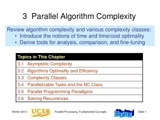
3 Parallel Algorithm Complexity • Review algorithm complexity and various complexity classes: • Introduce the notions of time and time/cost optimality • Derive tools for analysis, comparison, and fine-tuning Parallel Processing, Fundamental Concepts
3.1 Asymptotic Complexity Fig. 3.1 Graphical representation of the notions of asymptotic complexity. 3n log n = O(n2) ½ n log2n = W(n) 3n2 + 200n = Q(n2) Parallel Processing, Fundamental Concepts
Notation Growth rate Example of use f(n) = o(g(n)) strictly less than T(n) = cn2 + o(n2) f(n) = O(g(n)) no greater than T(n,m)=O(nlogn+m) f(n) = Q(g(n)) the same as T(n) = Q(n log n) f(n) = W(g(n)) no less than T(n,m) = W(n +m3/2) f(n) = w(g(n)) strictly greater than T(n) = w(log n) Little Oh, Big Oh, and Their Buddies < = > Parallel Processing, Fundamental Concepts
Some Commonly Encountered Growth Rates Notation Class name Notes O(1) Constant Rarely practical O(log log n) Double-logarithmic Sublogarithmic O(log n) Logarithmic O(logkn) Polylogarithmic k is a constant O(na), a < 1 e.g., O(n1/2) or O(n1–e) O(n/logkn) Still sublinear ------------------------------------------------------------------------------------------------------------------------------------------------------------------- O(n) Linear ------------------------------------------------------------------------------------------------------------------------------------------------------------------- O(n logkn) Superlinear O(nc), c > 1 Polynomial e.g., O(n1+e) or O(n3/2) O(2n) Exponential Generally intractable O(22n) Double-exponential Hopeless! Parallel Processing, Fundamental Concepts
Complexity History of Some Real Problems Examples from the book Algorithmic Graph Theory and Perfect Graphs [GOLU04]: Complexity of determining whether an n-vertex graph is planar Exponential Kuratowski 1930 O(n3) Auslander and Porter 1961 Goldstein 1963 Shirey 1969 O(n2) Lempel, Even, and Cederbaum 1967 O(n log n) Hopcroft and Tarjan 1972 O(n) Hopcroft and Tarjan 1974 Booth and Leuker 1976 A second, more complex example: Max network flow, n vertices, e edges: ne2 n2e n3 n2e1/2 n5/3e2/3 ne log2n ne log(n2/e) ne + n2+e ne loge/(n log n)n ne loge/nn + n2 log2+en Parallel Processing, Fundamental Concepts
3.2. Algorithm Optimality And Efficiency • Suppose that we have constructed a valid algorithm to solve a givenproblem of size n in g(n) time, where g(n) is a known function such as n log2n or n ²,obtainedthrough exact or asymptotic analysis. • A question of interest is whether or not the algorithmat hand is the best algorithm for solving the problem? Parallel Processing, Fundamental Concepts
3.2. Algorithm Optimality And Efficiency • Of course, algorithm quality can bejudged in many different ways,such as: • running time • resource requirements • simplicity (which affects the cost of development, debugging, and maintenance • portability What is the running timeƒ(n) of the fastest algorithm for solving this problem? Parallel Processing, Fundamental Concepts
3.2. Algorithm Optimality And Efficiency • If we are interested in asymptotic comparison, then because an algorithm with running timeg(n) is already known, ƒ(n) =O(g(n)); i.e., for large n, the running time of the bestalgorithm is upper bounded by cg(n) for some constant c. • If, subsequently, someonedevelops an asymptotically faster algorithm for solving the same problem, say in time h(n), we conclude that f(n)=O(h(n)). • The process of constructing and improvingalgorithms thus contributes to the establishment of tighter upper bounds for the complexity of the best algorithm Parallel Processing, Fundamental Concepts
3.2. Algorithm Optimality And Efficiency • On currently with the establishment of upper bounds as discussed above, we might workon determining lower bounds on a problem's time complexity. • A lower bound is useful as ittells us how much room for improvement there might be in existing algorithms. Parallel Processing, Fundamental Concepts
3.2. Algorithm Optimality And Efficiency • In the worst case, solution of the problem requires data to travel a certain distance or that a certain volume of data must pass through a limited bandwidth interface. An example of he first method is the observation algorithm on a p-processor square mesh needs at least 2p-2 communication steps in the worst case. (Diameter based lower bound) • The second method : is exemplified by the worst-case linear time required by any sorting algorithm on a binary tree architecture (bisection-based lower bound). Parallel Processing, Fundamental Concepts
3.2. Algorithm Optimality And Efficiency • In the worst case, solution of the problem requires that a certain number of elementary operations be performed. This is the method used forestablishing the Ω(n log n) lower bound for comparison-based sequential sortingalgorithms. • Showing that any instance of a previously analyzed problem can be converted to an instance of the problem under study, so that an algorithm for solving our problem can also be used, with simple pre and post processing steps, to solve the previous problem. Parallel Processing, Fundamental Concepts
3.2. Algorithm Optimality And Efficiency Lower bounds: Theoretical arguments based on bisection width, and the like Upper bounds: Deriving/analyzing algorithms and proving them correct Fig. 3.2 Upper and lower bounds may tighten over time. Parallel Processing, Fundamental Concepts
Some Notions of Algorithm Optimality Time optimality (optimal algorithm, for short) T(n, p) = g(n, p), where g(n, p) is an established lower bound Problem size Number of processors Cost-time optimality (cost-optimal algorithm, for short) pT(n, p) = T(n, 1); i.e., redundancy = utilization = 1 Cost-time efficiency (efficient algorithm, for short) pT(n, p) = Q(T(n, 1)); i.e., redundancy = utilization = Q(1) Parallel Processing, Fundamental Concepts
3.3. Complexity Classes • In complexity theory, problems are divided into several complexity classes according to their running times on a single-processor system (or a deterministic Turing machine, to be more exact). • Problems whose running times are upper bounded by polynomials in n are said to belong to the P class and are generally considered to be tractable. • Even if the polynomial is of a high degree, such that a large problem requires years of computation on the fastest available supercomputer. Parallel Processing, Fundamental Concepts
3.3. Complexity Classes • problems for which the best known deterministic algorithm runs in exponential time are intractable. For example, if solving a problem of size n requires the execution of 2n machine instructions, the running time for n= 100 on a GIPS (Giga IPS) processor will be around 400 billion centuries! A problem of this kind for which, when given a solution, the correctness of the solution can be verified in polynomial time, is said to belong to the NP (nondeterministic polynomial) class. Parallel Processing, Fundamental Concepts
3.3. Complexity Classes Figure 3.4. A conceptual view of complexity classes and their relationships Parallel Processing, Fundamental Concepts
3.4. Parallelizable Tasks And The NC Class parallel processing is generally of no avail for solving NP problems. A problem that takes 400 billion centuries to solve on a uniprocessor, would still take 400 centuries even if it can be perfectly parallelized over 1 billion processors. Again, this statement does not refer to specific instances of the problem but to a general solution for all instances. Thus, parallel processing is primarily useful for speeding up the execution time of the problems in P. Parallel Processing, Fundamental Concepts
3.4. Parallelizable Tasks And The NC Class Efficiently parallelizable problems in P might be defined as those problems that can be solved in a time period that is at most poly logarithmic in the problem size n, i.e.,T(p) = O(log k n) for some constant k, using no more than a polynomial number p =O(n l ) of processors. This class of problems was later named Nick’s Class (NC) in his honor. The class NC has been extensively studied and forms a foundation for parallel complexity theory. Parallel Processing, Fundamental Concepts
3.5 Parallel Programming Paradigms • Divide and conquer Decompose problem of size n into smaller problems; solve sub problems independently; combine sub problem results into final answer. T(n) =Td(n) +Ts+Tc(n) • Randomization When it is impossible or difficult to decompose a large problem into sub problems with equal solution times, one might use random decisions that lead to good results with very high probability. Example: sorting with random sampling • Approximation Iterative numerical methods may use approximation to arrive at solution(s). Example: Solving linear systems using Jacobi relaxation. Under proper conditions, the iterations converge to the correct solutions; more iterations greater accuracy Parallel Processing, Fundamental Concepts
3.5 Parallel Programming Paradigms The other randomization methods are: • Random search: When a large space must be searched for an element with certain desired properties, and it is known that such elements are abundant, random search can lead to very good average-case performance. 2. Control randomization: To avoid consistently experiencing close to worst-case performance with one algorithm, related to some unfortunate distribution of inputs, the algorithm to be applied for solving a problem, or an algorithm parameter, can be chosen at random. Parallel Processing, Fundamental Concepts
3.5 Parallel Programming Paradigms 3. Symmetry breaking: Interacting deterministic processes may exhibit a cyclic behavior that leads to deadlock (akin to two people colliding when they try to exit a room through a narrow door, backing up, and then colliding again). Randomization can be used to break the symmetry and thus the deadlock. Parallel Processing, Fundamental Concepts
3.6 Solving Recurrences In all examples below, ƒ(1) = 0 is assumed. f(n) = f(n – 1) + n {rewrite f(n – 1) as f((n – 1) – 1) + n – 1} = f(n – 2) + n – 1 + n = f(n – 3) + n – 2 + n – 1 + n . . . = f(1) + 2 + 3 + . . . + n – 1 + n = n(n + 1)/2 – 1 = Q(n2) This method is known as unrolling f(n) = f(n/2) + 1 {rewrite f(n/2) as f((n/2)/2 + 1} = f(n/4) + 1 + 1 = f(n/8) + 1 + 1 + 1 . . . = f(n/n) + 1 + 1 + 1 + . . . + 1 -------- log2 n times -------- = log2 n = Q(log n) Parallel Processing, Fundamental Concepts
More Example of Recurrence Unrolling f(n) = 2f(n/2) + 1 = 4f(n/4) + 2 + 1 = 8f(n/8) + 4 + 2 + 1 . . . = nf(n/n) + n/2 + . . . + 4 + 2 + 1 = n – 1 = Q(n) f(n) = f(n/2) + n = f(n/4) + n/2 + n = f(n/8) + n/4 + n/2 + n . . . = f(n/n) + 2 + 4 + . . . + n/4 + n/2 + n = 2n – 2 = Q(n) Parallel Processing, Fundamental Concepts
Still More Examples of Unrolling f(n) = 2f(n/2) + n = 4f(n/4) + n + n = 8f(n/8) + n + n + n . . . = nf(n/n) + n + n + n + . . . + n --------- log2 n times --------- = n log2n = Q(n log n) f(n) = f(n/2) + log2 n = f(n/4) + log2(n/2) + log2 n = f(n/8) + log2(n/4) + log2(n/2) + log2 n . . . = f(n/n) + log2 2 + log2 4 + . . . + log2(n/2) + log2 n = 1 + 2 + 3 + . . . + log2 n = log2 n (log2 n + 1)/2 = Q(log2n) Parallel Processing, Fundamental Concepts
Master Theorem for Recurrences Theorem 3.1: Given f(n) = a f(n/b) + h(n); a, b constant, h arbitrary function the asymptotic solution to the recurrence is (c = logb a) f(n) = Q(nc) if h(n) = O(nc – e) for some e > 0 f(n) = Q(nc log n) if h(n) = Q(nc) f(n) = Q(h(n)) if h(n) = W(nc + e) for some e > 0 Example:f(n) = 2f(n/2) + 1 a = b = 2; c = logba = 1 h(n) = 1 = O(n1 – e) f(n) = Q(nc) = Q(n) Parallel Processing, Fundamental Concepts
The End Parallel Processing, Fundamental Concepts