M 3 , WFD and POCIS
190 likes | 342 Views
Modeling of pesticide fate in a luxembourgish catchment with the Soil and Water Assessment Tool (SWAT) - combining modeling and monitoring. Stefan Julich 1& ² , Tom Gallé², Marion Frelat², Michael Bayerle², Hassanya El Khabbaz² & Denis Pittois²

M 3 , WFD and POCIS
E N D
Presentation Transcript
Modeling of pesticide fate in a luxembourgish catchment with the Soil and Water Assessment Tool (SWAT) - combining modeling and monitoring Stefan Julich1&² , Tom Gallé², Marion Frelat², Michael Bayerle², Hassanya El Khabbaz² & Denis Pittois² 1 TechnischeUniversitätDresden, Instit. for Soil Science & Site Ecology ² CRTE, CRP Henri Tudor - Luxembourg
M3, WFD and POCIS • M3 is a demonstration project for WFD policy implementation of the LIFE+ programme • M3 tests state-of-the-art monitoring and modelling tools for programme of measures (POM) evaluation • Can passive samplers (POCIS) help to validate and improve simulations of pesticide fate ?
Inroduction of study area elevation slope landuse Land use: ~ 30% managed pasture ~ 30% agriculture (corn, winter cereals, summer cereals) ~ 6% urban area
Emission modeling of pesticides Main challenges in model calibration • Monitoring data covering the dynamics of the emissionpathways/sources • Pesticide application date, amount, formulation and spatial distribution are unkown • Compound fateproperties t1/2 and KOC are spatially variable • Calibration atcatchmentoutlet, no distributed calibration possible t1/2 = 15 d Log KOC = 1.51
Case studyWark:Monitoring setup 4 6 3 5 2 1
The watershed • Warkwatershed ca. 82km² • First simulationconcentrate on Terbuthylazine • Applied on corn (~ 465 ha) • Statisticsindicate a applicationof340 g/ha on average • Same applicationdatefor all fields
Data Needs forpesticidefatemodelling ? • Whichcropsaregrown? • Whichsubstancesareapplied? • Whenarethepesticidesapplied? • Whatistheamountoftheapplication?
Loads – observed vs. simulated 4 6 3 5 2 1 • Event 1 toolessmobilization (surfacerunoff vs. Parameterization) • Event 2 viceversa
Floodwave 24/5-10/6 4 24/5-10/6 3 2 6 5 1
Loads – observed vs. simulated Mertzig 4 6 3 • Mertzigforbotheventstolessexport applicationamounts? • Niederfeulenfirsteventisunderestimated toolessmobilizationthroughsurfacerunoff? 5 2 Niederfeulen 1
Conclusions & outlook • Results indicate simulations do not match with the measurements • under or over estimation of surface runoff • POCIS measurement are useful to gain spatially distributed information of pesticide export to rivers • Comparison of simulation with POCIS results show the value of adequate Input Data like spatial information of application amounts and application times
Conclusions & outlook • Integration of more events in the model validation (measurements are still in progress) • Improve hydrological modelling • Simulate pesticide with spatially different application dates and amounts
Event loadswith long term POCIS 4 6 3 5 2 1
Performance of POCIS duringfloodwaves • Rsdetermined in the fieldwith composite samples over a day • Rs on different river sites RSD 20-30 % • No explanation for Rsvariability
Lossesduring longer exposure Memory test • Spiked POCIS exposed for differentlength of time in a river • Losses for compounds with log KOW <1 • ke: 0.04-0.1 d-1 (t1/2: 7-17 d) Exposure time
Loadcalculationbias • Loadcalculation on eventlevelbiasedonly on floodwave close to application