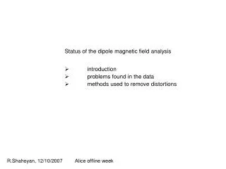
Status of the dipole magnetic field analysis introduction problems found in the data

Status of the dipole magnetic field analysis • introduction • problems found in the data • methods used to remove distortions R.Shahoyan, 12/10/2007 Alice offline week

Position 0 8cm 8cm 6.4cm Measure |Y| 36 cm Position 3 Position 1 Measure |Y| 36 cm y x IP z Position 2 Measurement layout 56.5 mm 56.5 mm 30 mm 30 mm (F.Bergsma) hall probes Back to IP Facing IP Z-steps of 6.4 or 8 cm -1392.8 <Z< -1047.2 -1058.3 <Z< -555.9

Coverage+ and – polarities have to be summed to minimize uncovered regions L3 Low L3 High

Data selection and cleaning • More than 1000 scans recorded, ~900 survive trivial selection cuts: empty/corrupted data, constant field etc. Part of selection was done by A.Morsch. • Probe-map (location of each probe ID on the vetronite plates) check. • Log-book and Scan Header information: Z coverage of each scan (~70 files have wrong labels for starting Z position), measuring head transverse location (wrong for ~20 scans), head position (wrong for ~100 scans) • Loss of probe ID’s : from time to time some probe ID’s are not correctly recorded. Recovered by matching to probe-unique calibration constants from the header (see L3 note ALICE-INT-2007-12) • Probes stability: in normal conditions probes measurements are reproducible on ~0.2 Gauss level and declared calibration precision (F.Bergsma) of ~1 Gauss holds (for most of them…). Nevertheless sometimes the probes record completely wrong values. • Consistency of field measured in different scans and by the FIP and BIP cards within the same scan: probes alignment (unique for given probe-map validity period) and scan-by-scan measuring head distortions (still not finished)

Probe-maps • Just 1 probe-map was provided, which failed to describe most of the data: • some probes mentioned in the map are not found in the data • instead the data contains the probes not mentioned in the map. • Such mismatches were corrected manually. In total, 4 different probe-maps were identified (after that the records of the 2nd one were found, confirming already identified map)

Probe-maps Example of the probe (#188) not fitting to other measurements when taken at its declared position. Need to reassign the probe position to make its measurement consistent with other data. BZ BX

Probe-maps Example of successful probe matching: Probe #100 mentioned in the probe-map is not found in the data. Instead, data sees probes #195 and #123 not mentioned in theprobe-map. Probe #123 is found to match the field expected where #100 should be (check is done for multiple Z positions) #100  #123 Z step 0

Probe-maps #69  #195 ambiguous Probe #195 is found to match the field expected where #69 should be unambiguous

Probe-maps #57 Declared probe #125 is not foundin the data. Instead #57 is found, but its values don't match to field of other probes. Tried to find matching probe by using different probe ID’s not involved in measurements. No probe is found to match at all Z’s  the “correct probe” is not calibrated

Data quality BTOT BTOT Probes calibration is in general very good ( 1Gauss) but there are a few ones which show 3-4 Gauss deviations from the expected field

Data quality Some probes suddenly change their sign. Comparison of their inverted measurements with the field measured by their neighbors show that apart from the sign flip the calibration is also lost. In worst case (#119) such behaviour is observed in ~20% of scans. FIPBIP

Data quality BX BY From time to time some probes measure completely wrong field just for a few Z-steps. ~ in half of cases such behaviour is associated with anomalous temperature. Tracked by visual inspection of each data measurement, the anomalous values are excluded from the analysis 

Data quality In some scans the sign of the field measured by different probes gets random (cabling?). FIPBIP

Data taking conditions information Lot of files with measuring head location wrongly recorded. Part of problematic data was fixed by A.Morsch. Sometimes trivial to track down since the mentioned coordinates are not possible but often the comparison with other measurements is needed. For ~10% of the data the head orientation is wrong (13)

Difference between various data sets (same probes, same head orientation/position) BTOT is reproduced on the level <4 Gauss. Similar differences are observed between the data for opposite polarities. 10-3

Compatibility of measurements by FIP and BIP plates All scans show systematic differences between the measurements by the FIP and BIP probes in the same location (even for the total field, which should be robust against the probes rotations) FIPBIP Rotations?Shifts?Calibration?

Model to fit the field distortions Field seen by the 3D probe in its local frame ( lab.frame for FIP probes in position 0): - rotation matrix bringing vector from lab to local frame - rotation matrix accounting the probe’s inclinations wrt its ideal position on the plate - gradients of field components in lab. frame(calculated numerically from the difference of neighboring measurements for the dominant components and exploring and for minor ones - vector of probe’s displacements wrt its ideal position - vector of residual miscalibration  Difference between the local measurement and the reference value (other probe): (1)

Correcting distortions FIPBIP Fit to (1) shows some improves consistency of FIP and BIP measurements, but not always (almost no effect at all for the last period of data taking, when the probes fixation was improved)

Correcting distortions FIPBIP Fit to (1) shows some improves consistency of FIP and BIP measurements, but not always (for last period of data taking, when the probes fixation was improved almost no effect at all) The field gradients are quite strong (reaching > 100 Gauss/cm)

probe 1 probe 3 30 mm probe 2 glass cube (4x4x2.5 mm) • Probes are not point-like :  their size does matter! • Different components are measured at different space points. • Probes on the BIP plate are not measuring the same points as their partners on FIP, even in case of ideal alignment

Correcting distortions FIPBIP Modify fit model to account for the individual displacement of 1D probe for each projection preliminary

Correcting distortions y ~17 mrad relative tilt between FIP and BIP plates x z Example of obtained rotations and miscalibrations probe-map valid for the majority of scans: 19 Aug–10 Sep(0 means that fit/comparison is not possible :one of the FIP/BIP probes is missing) NOTE: these fits show only the relative alignment between the pairs of FIP and BIP probes

Correcting distortions Example of obtained rotations and miscalibrations (last probe-map: 9-23 Oct. : probes were readjusted) The common tilt has been removed

Correcting distortions Example of obtained offsets for each 1D probe (last probe-map: 9-23 Oct)

Correcting distortions • How the absolute probes/plates alignments wrt lab system can be done?(work in progress) • To do this we need to know the “reference” correct field at least in some restricted region. • Suppose we are able to describe the distorted field on the surface of the volume by the solution of the Laplace equation. • Explore the fact that : • both “distorted fitted” and correct fields are the solutions of the Laplace equation  their difference (“fake field”)too. • the solution of the Laplace equation has its extremum on the surface of the volume  • As we go further from the surface inside the volume the error (“fake field”) may only decrease  the fitted field becomes closer to the correct field. •  • Do few iterations by minimizing (as a function of the alignment parameters) the difference between the distortedmeasurements deep in the volume and the fitted field.

Field parameterization method (based on H.Wind, NIM 84 (1970) 117) • In the absence of currents all magnetic field components and scalar potential must obey Laplace equation ,  fully defined by their values on the volume surface. • The general solution in Cartesian coordinates for the box with sides X,Y and Z is: • (1) • Since the field main component (BX for Alice dipole) is the most robust against the measurements errors, one can • fit BX values measured on the surface of the box to (1) • integrate along X to obtain the  • compute the field inside the volume as • Caveats: • for the fit to be convergent, the measurements should be done in the points equidistant in each dimension (no missing points are allowed). • since the  is obtained by integrating in one dimension, it is precise up to a function of two other dimensions (also obeying to 2D Laplace equation): • These missing functions must be obtained by fitting the difference between the measured and calculated minor components to 2D version of (1).

Field parameterization Data with 12 kA and 30 kA in L3 were taken with both polarities, but the coverage by each polarity is quite incomplete.

Field parameterization Data with 12 kA and 30 kA in L3 were taken with both polarities, but the coverage by each polarity is quite incomplete.Need to take together + and – (inverting the field) currents data to improve the coverage.This allows to define large enough rectangular surfaces for the potential reconstruction (only 30kA is shown) Missing points are filled using splines

Comparison of data (averaged over different scans) with calculation CalculationData X dependence Center of the dipolebox positions: 1 and 3 Data – Calc. CalculationData Above the centerbox positions: 0 and 2 Data – Calc.

Comparison of data (averaged over different scans) with calculation CalculationData Y dependence Data – Calc. Z dependence CalculationData Data – Calc.

Comparison of individual measurements with calculation (Y=36 cm, Z=-853) There are apparent systematic differences between the deviations of measurements with different plates orientations: still to be seen if they are scan dependent

Very preliminary: example of minimization of the differences between the data and the fitted field (probe size is not accounted) Before After Data – Fit (for points 24 cm from the surface in X and Y and 80 cm in Z)

Summary • Lot of problems with data quality and the information on data taking conditions, seem to be mostly solved  All probe-maps are identified  Data are cleaned  Effects caused by the finite probe’s size are accounted (still have to do some check on compatibility of the offsets obtained by the measurements with different measuring head orientations) • The field parameterization routines are working • The probes alignment is being done Tentative time estimate to get the field map for the measured data and filling the uncovered regions by Tosca calculations: ~ 1 month (if no new problem found)

Failed attempt of probes alignment exploring Biot-Savart law • Fit deviation of from 0 for all possible plaquets as a function of probe’s misalignments… • Fails because even in the case of the ideal alignment such rough computed on the loop of 4 points is far from 0 due to the non-linearity of the field. • Tried to account for this by subtracting the calculating by Tosca, but itdid not work because: • Tosca does not respect Maxwell equations with needed precision. • Used too crude mesh leads to field fluctuations on the level of a few Gauss...

The only complete probe map (used for ~30 very short scans)

Status of the dipole magnetic field analysis introduction problems found in the data