Download
1 / 55
550 likes | 675 Views
Recombination and Linkage. The genetic approach. Start with the phenotype; find genes the influence it. Allelic differences at the genes result in phenotypic differences. Value: Need not know anything in advance. Goal Understanding the disease etiology (e.g., pathways)

E N D
The genetic approach • Start with the phenotype; find genes the influence it. • Allelic differences at the genes result in phenotypic differences. • Value:Need not know anything in advance. • Goal • Understanding the disease etiology (e.g., pathways) • Identify possible drug targets
Approaches togene mapping • Experimental crosses in model organisms • Linkage analysis in human pedigrees • A few large pedigrees • Many small families (e.g., sibling pairs) • Association analysis in human populations • Isolated populations vs. outbred populations • Candidate genes vs. whole genome
Advantages If you find something, it is real Power with limited genotyping Numerous rare variants okay Disadvantages Need families Lower power if common variant and lots of genotyping Low precision of localization Linkage vs. association
Outline • Meiosis, recombination, genetic maps • Parametric linkage analysis • Nonparametric linkage analysis • Mapping quantitative trait loci
Genetic distance • Genetic distance between two markers (in cM) = Average number of crossovers in the interval in 100 meiotic products • “Intensity” of the crossover point process • Recombination rate varies by • Organism • Sex • Chromosome • Position on chromosome
Crossover interference • Strand choice • Chromatid interference • Spacing • Crossover interference • Positive crossover interference: • Crossovers tend not to occur too • close together.
Recombination fraction We generally do not observe the locations of crossovers; rather, we observe the grandparental origin of DNA at a set of genetic markers. Recombination across an interval indicates an oddnumber of crossovers. Recombination fraction = Pr(recombination in interval) = Pr(odd no. XOs in interval)
Map functions • A map function relates the genetic length of an interval and the recombination fraction. r = M(d) • Map functions are related to crossover interference, but a map function is not sufficient to define the crossover process. • Haldane map function: no crossover interference • Kosambi: similar to the level of interference in humans • Carter-Falconer: similar to the level of interference in mice
Before you do anything… • Verify relationships between individuals • Identify and resolve genotyping errors • Verify marker order, if possible • Look for apparent tight double crossovers, indicative of genotyping errors
Parametric linkage analysis • Assume a specific genetic model. For example: • One disease gene with 2 alleles • Dominant, fully penetrant • Disease allele frequency known to be 1%. • Single-point analysis (aka two-point) • Consider one marker (and the putative disease gene) • = recombination fraction between marker and disease gene • Test H0: = 1/2 vs. Ha: < 1/2 • Multipoint analysis • Consider multiple markers on a chromosome • = location of disease gene on chromosome • Test gene unlinked ( = ) vs. = particular position
Missing data The likelihood now involves a sum over possible parental genotypes, and we need: • Marker allele frequencies • Further assumptions: Hardy-Weinberg and linkage equilibrium
More generally • Simple diallelic disease gene • Alleles d and + with frequencies p and 1-p • Penetrances f0, f1, f2, with fi = Pr(affected | i d alleles) • Possible extensions: • Penetrances vary depending on parental origin of disease allele f1 f1m, f1p • Penetrances vary between people (according to sex, age, or other known covariates) • Multiple disease genes • We assume that the penetrances and disease allele frequencies are known
Likelihood calculations • Define g = complete ordered (aka phase-known) genotypes for all individuals in a family x = observed “phenotype” data (including phenotypes and phase-unknown genotypes, possibly with missing data) • For example: • Goal:
The parts • Prior = Pop(gi) Founding genotype probabilities • Penetrance = Pen(xi | gi) Phenotype given genotype • TransmissionTransmission parent child = Tran(gi | gm(i), gf(i)) Note: If gi = (ui, vi), where ui = haplotype from mom and vi = that from dad Then Tran(gi | gm(i), gf(i)) = Tran(ui | gm(i)) Tran(vi | gf(i))
The likelihood Phenotypes conditionally independent given genotypes F = set of “founding” individuals
That’s a mighty big sum! • With a marker having k alleles and a diallelic disease gene, we have a sum with (2k)2nterms. • Solution: • Take advantage of conditional independence to factor the sum • Elston-Stewart algorithm: Use conditional independence in pedigree • Good for large pedigrees, but blows up with many loci • Lander-Green algorithm: Use conditional independence along chromosome (assuming no crossover interference) • Good for many loci, but blows up in large pedigrees
Ascertainment • We generally select families according to their phenotypes. (For example, we may require at least two affected individuals.) • How does this affect linkage? If the genetic model is known, it doesn’t: we can condition on the observed phenotypes.
Model misspecification • To do parametric linkage analysis, we need to specify: • Penetrances • Disease allele frequency • Marker allele frequencies • Marker order and genetic map (in multipoint analysis) • Question: Effect of misspecification of these things on: • False positive rate • Power to detect a gene • Estimate of (in single-point analysis)
Model misspecification • Misspecification of disease gene parameters (f’s, p) has little effect on the false positive rate. • Misspecification of marker allele frequencies can lead to a greatly increased false positive rate. • Complete genotype data: marker allele freq don’t matter • Incomplete data on the founders: misspecified marker allele frequencies can really screw things up • BAD: using equally likely allele frequencies • BETTER: estimate the allele frequencies with the available data (perhaps even ignoring the relationships between individuals)
Model misspecification • In single-point linkage, the LOD score is relatively robust to misspecification of: • Phenocopy rate • Effect size • Disease allele frequency However, the estimate of is generally too large. • This is less true for multipoint linkage (i.e., multipoint linkage is not robust). • Misspecification of the degree of dominance leads to greatly reduced power.
Other things • Phenotype misclassification (equivalent to misspecifying penetrances) • Pedigree and genotyping errors • Locus heterogeneity • Multiple genes • Map distances (in multipoint analysis), especially if the distances are too small. All lead to: • Estimate of too large • Decreased power • Not much change in the false positive rate Multiple genes generally not too bad as long as you correctly specify the marginal penetrances.
Software • Liped ftp://linkage.rockefeller.edu/software/liped • Fastlink http://www.ncbi.nlm.nih.gov/CBBresearch/Schaffer/fastlink.html • Genehunter http://www.fhcrc.org/labs/kruglyak/Downloads/index.html • Allegro Emailallegro@decode.is • Merlin http://www.sph.umich.edu/csg/abecasis/Merlin
Nonparametric linkage Underlying principle • Relatives with similar traits should have higher than expected levels of sharing of genetic material near genes that influence the trait. • “Sharing of genetic material” is measured by identity by descent (IBD).
Identity by descent (IBD) Two alleles are identical by descent if they are copies of a single ancestral allele
IBD in sibpairs • Two non-inbred individuals share 0, 1, or 2 alleles IBD at any given locus. • A priori, sib pairs are IBD=0,1,2 with probability 1/4, 1/2, 1/4, respectively. • Affected sibling pairs, in the region of a disease susceptibility gene, will tend to share more alleles IBD.
Example • Single diallelic gene with disease allele frequency = 10% • Penetrances f0 = 1%, f1 = 10%, f2 = 50% • Consider position rec. frac. = 5% away from gene
Complete data case Set-up • n affected sibling pairs • IBD at particular position known exactly • ni = no. sibpairs sharing i alleles IBD • Compare (n0, n1, n2) to (n/4, n/2, n/4) • Example: 100 sibpairs (n0, n1, n2) = (15, 38, 47)
Affected sibpair tests • Mean test Let S = n1 + 2 n2. Under H0: = (1/4, 1/2, 1/4), E(S | H0) = n var(S | H0) = n/2 Example: S = 132 Z = 4.53 LOD = 4.45
Affected sibpair tests • 2 test Let 0 = (1/4, 1/2, 1/4) Example: X2 = 26.2 LOD = X2/(2 ln10) = 5.70
Incomplete data • We seldom know the alleles shared IBD for a sib pair exactly. • We can calculate, for sib pair i, pij = Pr(sib pair i has IBD = j | marker data) • For the means test, we use in place of nj • Problem: the deminator in the means test, is correct for perfect IBD information, but is too small in the case of incomplete data • Most software uses this perfect data approximation, which can make the test conservative (too low power). • Alternatives: Computer simulation; likelihood methods (e.g., Kong & Cox AJHG 61:1179-88, 1997)
Larger families Inheritance vector, v Two elements for each subject = 0/1, indicating grandparental origin of DNA
Score function • S(v) = number measuring the allele sharing among affected relatives • Examples: • Spairs(v) = sum (over pairs of affected relatives) of no. alleles IBD • Sall(v) = a bit complicated; gives greater weight to the case that many affected individuals share the same allele • Sall is better for dominance or additivity; Spairs is better for recessiveness • Normalized score, Z(v) = {S(v) – } / • = E{ S(v) | no linkage } • = SD{ S(v) | no linkage }
Combining families • Calculate the normalized score for each family Zi = {Si – i} / i • Combine families using weights wi ≥ 0 • Choices of weights • wi = 1 for all families • wi = no. sibpairs • wi = i(i.e., combine the Zi’s and then standardize) • Incomplete data • In place of Si, use where p(v) = Pr( inheritance vector v | marker data)
Software • Genehunter http://www.fhcrc.org/labs/kruglyak/Downloads/index.html • Allegro Emailallegro@decode.is • Merlin http://www.sph.umich.edu/csg/abecasis/Merlin
ANOVA at marker loci • Split mice into groups according to genotype at marker • Do a t-test / ANOVA • Repeat for each marker
Humans vs Mice • More than two alleles • Don’t know QTL genotypes • Unknown phase • Parents may be homozygous • Markers not fully informative • Varying environment