Download
1 / 20
220 likes | 522 Views
MARGINAL COST AND SECOND-BEST PRICING FOR WATER SERVICES. H. Youn Kim Presented by Adekunle Dada. INTRODUCTION. Regulatory commissions faced with maintaining ideal pricing structure. Average cost pricing, AC = P. Profit maximizing Marginal cost pricing, MC = P. Welfare maximizing .

E N D
MARGINAL COST AND SECOND-BEST PRICING FOR WATER SERVICES H. Youn Kim Presented by Adekunle Dada
INTRODUCTION • Regulatory commissions faced with maintaining ideal pricing structure. • Average cost pricing, AC = P. Profit maximizing • Marginal cost pricing, MC = P. Welfare maximizing. • Devise second best pricing rules .
PURPOSE OF STUDY • Estimate marginal cost and apply the second best pricing for water services. • Water Utility viewed as multiproduct firm Residential and Nonresidential services. • Translog multiproduct cost funstion.
Marginal cost equation and Second best pricing rules • lnC = Where C = Using Shephard’s Lemma to get cost share equations: Where This is the total cost accruing to input j.
Equations (contd) • Cost elasticity of output used in deriving marginal cost : • and i = R, N Thus = • Degree of overall scale economies for the multiproduct firm SL is defined as the reciprocal of the sum of cost elasticities of individual outputs (Baumol, Panzar and Willig 1982) • Ratio of total production cost is equal to total revenue.
Inadequacy of MC pricing • If SL > 1, economies of scale If SL = 1, constant returns to scale If SL < 1, diseconomies of scale • Economies of scale exist only if revenue yielded from MC pricing falls short of TC • Diseconomies exist if TR exceeds TC • CRTS exist if TR equals TC MC pricing cannot be used for a firm operating under conditions of economies of scale as it pertains to financial viability. Example: Water Utilities with large FC but small MC.
Subsidy • So if D = subsidy D(YR, YN) = C(YR, YN) – R(YR, YN) Recall SL = C/R, then R = C/SL Thus D(YR, YN) = C(YR, YN) – C(YR, YN)/S = C(YR, YN)(1 – 1/SL) • If SL is large then subsidy must be large • If SL is close to 1 (CRTS) subsidy and MC pricing may be a viable policy alternative • If SL < 1 then unsubsidized marginal cost pricing is feasible.
Maximizing Social Welfare • Suppose water supply firm faces budget or profit constraint: Max V( PR, PN, I) IUF St PRYR + PNYN – C(YR, YN) = B Soln: (PR – MCR)/PR= ηNN – ηRN (PR – MCR)/PNηRR - ηNR ηNN & ηRR – own price elasticities of demand for nonresidential and residential water. ηNR &ηRN – cross price elasticity is zero since residential is independent of nonresidential output. Thus: PR – MCR = PN – MCN PR *ηNN PN *ηRR
Welfare loss • The amount by which price diverges from MC for each output is inversely proportional to the elasticity of demand. • If ηRR <1, PR – MCR is large This is reduction in welfare loss • Overhead expenses for services produced with economies of scale are best covered with revenues from the more inelastic part of service.
DATA AND ESTIMATION Cross section of 60 water utilities collected during the survey of water utilities by US environmental protection agency in 1973 • Cost shares are calculated by dividing cost attributable to each input by TC • Output is measured in terms of amount of water treated in millions of gallons per day. • Price of labor is obtained by dividing gross payroll by number of yearly man-hours. • Price of energy measured by dividing total power expenditures by yearly kilowatt hour usage. • Price is capital computed by considering interest rate on long term debt and depreciation rate. • Capacity utilization measured by load factor for water system. • Service distance measured by miles of distribution pipelines.
RESULTS AND DISCUSSION • The parameter estimates of the translog multiproduct cost function from table one are used to derive estimates of cost elasticities of outputs and marginal costs of outputs.
Overall Economies of Scope and Scale • Economies of scope (Baumol, Panzar and Willig, 1982) measures % cost increase due to joint production of residential and nonresidential services. • Cost elasticity of residential output is estimated by ɛCR = 0.53037 - 0.42487lnYR + 0.10086lnYN + 0.08885lnWL - 0.11238lnWK + 0.02353lnWE- 0.59305lnZU +0.44056lnZM • Cost elasticity of nonresidential output is given by ɛCN =0.25741 + 0.10086lnYR + 0.14868lnYN - 0.02182lnWL + 0.01496lnWK + 0.00686lnWE + 0.13495lnZU – 0.32537lnZM • Overall cost elasticity obtained by summing both cost elasticities is ɛCY =0.78778 – 0.32401lnYR + 0.24954lnYN + 0.06703lnWL – 0.09742lnWK + 0.03039lnWE – 0.45810lnZU + 0.11519lnZM
Degree of scale economics is the inverse of overall cost elasticity. • Effects of relative price movement of labor, capital and energy are generally small relative to effects of outputs, capacity utilization and service distance. • Economies of scale are largely determined by levels of output, capacity utilization and service distance.
Small utilities exhibit marked economies of scale while large utilities exhibit moderate diseconomies of scale. Small utilities cannot adopt MC pricing as it would lead to financial insolvency.
Marginal cost elasticities of output, input prices and operating variables.% change in MC of residential and nonresidential output due to change in variables.Substantial effect of operating variables on MCs of water supply.
Price-marginal cost margins for residential and nonresidential are greater than zero. Residential water service priced 158% above MC.Nonresidential priced 40% above MC.Price discrimination seems to be favor nonresidential users.
Second best prices are only slightly higher than prices actually charged.% change from residential water price to second best is 0.10. For nonresidential, it is 0.09.Thus, the move to the calculated optimal rates requires a 10% increase for residential customers and a 9% increase for nonresidential customers.
SUMMARY AND CONCLUSION • Discussed implication of MC pricing. • Examined second best pricing scheme. • While existing price structure is different from MC, it does not appear to deviate substantially from second best optimum. • This study is significant to regulators, policy makers and water supply managers.
THANK YOU FOR LISTENING No questions please.