well

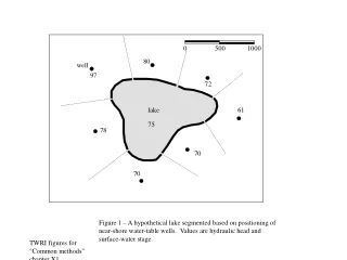
1. 0 500 1000 80 well 97 72 lake 61 75 78 70 70 Figure 1 – A hypothetical lake segmented based on positioning of near-shore water-table wells. Values are hydraulic head and surface-water stage.

2. 0 500 1000 80 well 200 97 72 425 650 225 500 550 430 lake 61 350 850 800 75 78 400 275 70 600 300 70 Figure 1 – including dimensions.

3. water-table well shoreline segment Lake m break in slope A ground-water flow lines t L outside of local flow domain flow passes beneath lake and is Figure 2 –Typical hydraulic conditions in the vicinity of the shoreline of a surface-water body.

4. 1000 0 500 80 well 72 97 lake 75 61 hinge line 78 70 70 Figure 3 – A flow net generated to indicate flow of water to and from a hypothetical lake. Ground-water flow direction is indicated by flowlines (solid lines) and lines of equal hydraulic head (equipotential lines) are shown with dashed lines. Values shown are hydraulic head and surface-water stage.

5. 1000 0 500 80 well 72 97 lake 75 61 hinge line 78 70 70 Figure 3 – alternate.

6. 80 well 72 97 B A C lake 75 D 61 G hinge line E 78 70 F 70 Figure 4 – Conceptualization of flow based on flow-net analysis and segmented Darcy fluxes. The position of the hinge line changes depending on the method used.

7. Figure 5 – Hydraulic potentiomanometer (HPM) showing drive well inserted into lakebed and manometer indicating a very small vertical hydraulic-head gradient. (Photo by Don Rosenberry)

8. Figure 6 – Components of the HPM system. (from Winter et al., 1988)

9. Figure 7 – Hydraulic potentiomanometer designed to place the manometer tubes connected to the drive probe and to the surface-water body close together to minimize out-of-level errors. (Photo by Jim Lundy)

10. Figure 8 – HPM potentioprobe with drive hammer, shown driven about 2 m beneath the lakebed. Manometer and hand-crank peristaltic pump are visible in background. (photo by Don Rosenberry)

11. Figure 9 – Hydraulic potentiomanometer (created by Joe Magner, Minnesota Pollution Control Agency) with manometer connected to drive probe. Note the proximity of the lake and drive-probe tubes to minimize out-of-level errors. Note also the in-line water bottle to keep the vacuum pump dry. (Photo by Don Rosenberry)

12. Figure 10 – HPM device consisting of a commercially available retractable soil-gas vapor probe connected to threaded pipe with tubing inside the pipe connected to the vapor probe, and a separate tube taped to the outside of the pipe that extends to the lake water surface. (Photo by Don Rosenberry)

13. Figure 11 – Potentioprobe constructed from a commercially available root feeder with the coiled tubing substituting for a manometer (from Wanty and Winter, 2000).

14. Figure 12 – MHE PP27 probe used to indicate difference in head (Henry, 2000). (Photo by Mark Henry)

15. Figure 13 – Half-barrel seepage meter (from Lee and Cherry, 1978). The top panel shows typical installation with bag inserted to a tube inserted through a rubber stopper. The bottom panel shows installation in shallow water with vent tube to allow trapped gas to escape.

16. Figure 14 – Seepage meter modified for use in large lakes (from Cherkauer and McBride, 1988).

17. Figure 15 – Seepage meter modified for use in deep water (from Boyle, 1994). 62 cm

18. Figure 16 – Plastic bag attached to a garden-hose shut-off valve. Bag is filled with a known volume of water and then purged of air. Valve is closed. Bag is threaded onto male threads on seepage meter and valve then is opened to begin seepage measurement. (Photo by Donald Rosenberry)

19. 226 0 56 113 169 282 339 Seepage flux through standard half-barrel meter, in cm d-1 Figure 17 – Resistance to flow related to tubing diameter and rate of seepage. Seepage flux assumes a 0.25 m2-area seepage meter (modified from Fellows and Brezonik, 1980).

20. SEEPAGE FLUX, in m/s x 10-8 Figure 18 – Seepage flux measured at two seepage meters located 1 m apart. Flux values are in m/s (from Shaw and Prepas, 1990).