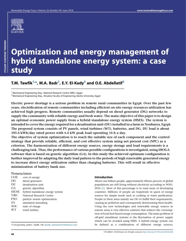
Optimization and energy management of hybrid standalone energy system: a case study
Optimization and Energy Management of Hybrid Standalone Energy System: A Case Study T.M. Tawfik*, M.A. Badr*, E.Y. El-Kady**, O.E. Abdellatif** *Mechanical Engineering Dep., National Research Centre (NRC) ** Mechanical Engineering Dep., Shoubra Faculty of Engineering, Banha University Abstract Electric power shortage is a serious problem in remote rural communities in Egypt. Over the past few years, electrification of remote communities including efficient on-site energy resources utilization has achieved high progress. Remote communities usually depend on diesel generator (DG) networks to supply the community with reliable energy and fresh water. The main objective of this paper is to design an optimal economic power supply from a hybrid standalone energy system (HSES). The system is intended to cover the energy required for a desalination unit (DU) installed in a farm in Noubarya, Egypt. The proposed system consists of PV panels, Wind Turbines (WT), Batteries, and DG. DU load is about 105.6 kWh/day rated power with 6.6 kW peak load operating 16 hours a day. The objective of system optimization is to reach the suitable size of each component and the control strategy that provide reliable, efficient, and cost effective system using net present cost (NPC) as a criterion. The harmonization of different energy sources, energy storage and load requirements is a challenging task. Thus, the performance of various possible configurations is investigated, using iHOGA software that is based on genetic algorithm (GA). In this study the achieved optimum configuration is further improved by adapting the daily load pattern to the periods of high renewable generated energy to increase direct energy utilization rather than charging batteries. This will result in effective minimization of battery bank size. Keywords: Hybrid system; iHOGA; Optimization; Energy management; Renewable energy Nomenclature COE: cost of energy DG: diesel generator DU: desalination unit GA: genetic algorithm HESE: hybrid standalone energy system NRC: National Research Centre PSO: particle swarm optimization SA: simulated annealing SOC: state of charge WT: Wind Turbine 1. Introduction About one billion people; approximately fifteen percent of global populations are still living without electricity according to WEO- 2016 [1]. Most of this percentage is in rural areas of developing countries. Millions of people hopelessly in quest of energy sources for simple needs such as cooking or water purification. People in these areas mainly use DG to fulfill their requirements, causing air pollution and consequently deteriorating their health. Using the new technologies and renewable energy sources in remote areas is very effective solution that reduces the consumption of fossil fuel-based energy consumption. The main problem of off-grid standalone systems is the fluctuation of power supply which can be avoided using HSES. A hybrid energy system can be defined as a combination of different energy sources; renewable/convention energy. Recently, the application of HSES has increased steadily as a suitable solution for rural remote areas. There have been a number of researches carried out in this field over the last few decades. M. Uzunoglu et-al, [2] presented a review of the optimization techniques for HES sizing within minimum investment and operating cost. The studied techniques are (GA), particle swarm optimization (PSO), simulated annealing (SA) and HOMER. The selection of sizing approach depended on user demand, availability of renewable resources and climatic conditions. Lanre Olatomiwa et-al, [3], focused on the various approaches and techniques that can be used to develop a successful energy management strategy; for both standalone hybrid renewable energy systems and the grid-connected hybrid renewable systems, such as "energy management based on linear programming, intelligent techniques and also energy management by fuzzy logic controller". This paper showed that selecting the suitable energy management strategy is essential to control the energy flow between various components of the energy system that increases the system reliability, decreases electricity shortage, reduces the COE and increases the system component lifetime. Monowar Hossaina et-al, [4] presented a hybrid stand-alone renewable energy system that comprises of PV, WT, DG, converter and battery for a touristic resort in South China Sea, Malaysia which fully depends on diesel generators as a power supply. The resort estimated peak and average load per day were 1185 kW and 13,048 kW respectively. HOMER software was used for economic and technical analysis of the system. The results showed that the hybrid system have lower NPC and COE than the diesel only system. Lanre Olatomiwa et-al, [5] studied the feasibility of different power generation configurations comprising PV, WT and DG in six geo-political zones of Nigeria. Seven system configurations including: stand-alone DG only system, PV/DG, PV/DG/battery, WT/DG, WT/DG/battery, PV/WT/DG and PV/WT/DG/battery, were investigated; also by HOMER, to determine the most economically feasible solution based NPC, COE and renewable fraction (RF). The result showed that the PV/DG/battery hybrid renewable system configuration is found to be the optimum configuration in cases of 1.1 and $1.3/l of diesel fuel. It also displayed better performance in fuel consumption and CO2 reduction. The best optimum location to install this system was in Tambo village in the tropical dry climatic zone and the overall results indicated that system configurations perform better with regards to the NPC for all six simulations, generated energy, fuel consumption and CO2 reduction. Alam et-al, [6] presented a design of a hybrid WT/PV/Fuel cell power system with battery for remote area. A fuzzy logic power flow controller has been proposed to provide continuous power based on the economic power generation of preliminary analysis. A 20 kW Wind turbine and 80 kW PV array with 10 kW fuel cell was used in the simulation. Excess power was directed to the batteries first and then to electrolyzer. The results showed that the optimum system has 254 kWh/yr unmet load which represented a high percentage of the total load. The cost of energy is estimated to be 1.045 $/kWh which is very high. Therefore the system needs to be improved for better reliable performance. A comparison between grid supply, PV system, and wind power system was presented by [7]. The results of this study considered the renewable systems to be more expensive than the grid supply. Using a multi-sources renewable energy system (hybrid energy system) instead of a single source system would improve the renewable systems economics and reliability. This could be further improved using energy storage device to utilize the excess energy. Ajao et-al, [8] performed an economic analysis of PV-WT system for a Nigerian area. The authors concluded that the proposed system is expensive because of high capital and installation costs. In this study, reduction of greenhouse gas emission wasn't taken in account to improve the cost-effectiveness of the system would be if the system was designed for remote areas. Getachew Bekele et-al, [9] focused on the possibility of supplying electricity to 200 household in rural remote area in Ethiopia using HSES. In this case, HOMER software had been used for the evaluation purpose. Moreover, the effects of wind speeds, PV costs and diesel prices on the optimization solutions were studied. The results showed the most cost effective combination is PV, DG and battery using load following strategy. The authors concluded that the study results could be considered applicable for the regions that have similar climatic conditions. Feasibility analysis of hybrid renewable energy system (HRES) for a village in Bangladesh far from grid was presented by Himadry Shekhar Das, et-al [10]. HOMER program had been used for simulating the system using site weather data and load profile of 50 families (annual average load is 213 kWh/day). Sensitivity analysis has also been carried out to determine the best suitable system in case of future change of the parameters. The results showed that the feasible system for this location and load profile is PV-WT-Battery. The optimum system had a total NPC of 224,345 $ and COE of 0.161 $/kWh with no CO2 emission (in the current work, the obtained COE less than 0.15). The sensitivity analysis also proved that HRES could cover any expected increase in load in the future. Also Md. Mustafizur Rahman et-al, [11] suggested seven scenarios of combining HSES to minimize the economic and environmental impact. The suggested scenarios were (100%, 80%, 60%, 50%, 35%, 21% and 0%) renewable fraction. A case study for the remote community in Canada was conducted. The aim of this study was also finding the best combination of HSES from the available resources for off-grid location. Using HOMER software the results showed that 80% renewable energy scenario could achieve the optimum techno-economic demand while using 72% scenario obtained higher COE.In a similar study M. Fadaeenejad et-al, [12] presented an analysis and optimization for a HSES which designed for rural electrification in Malaysia. The evaluation of the optimization fulfilled using IHOGA. The reached results illustrated that the wind energy is used as a supportive source of energy and the HSES are cost effectively for this rural area. Similarly, Anita Gudelj et-al, [13] optimized the size of HSES minimizing the NPC and the pollutant emissions using iHOGA. The results showed that the PV-WT-battery system had considerable reductions in CO2 emission and NPC while using DG as a back-up source improved system reliability diminishing shortage. J. B. Fulzele et-al, [14] focused on finding the optimum hybrid energy system (HES) which is economically feasible subject to physical and operational constraints and strategies. The system was designed to feed a load which had seasonal variations. The system has been simulated and optimized using iHOGA. The main goal of optimization was to select the best combination of components to satisfy the constraints and minimizes NPC. The results showed that the system covered the required load with only 1% shortage. The results of this study didn't take into consideration that the excess energy was about 25% and minimizing this value would reduce the cost of energy (COE). Designing and optimizing HSES necessitates the choice of the suitable combination of energy components and establish the optimum control strategy to manage the system that would be reliable and economical over the system life time. Over sizing the system would result high initial cost, while small size system could result in energy. This paper presents the design of an optimized HSES consisting of PV, WT, battery bank and DG as a backup for supplying electricity to water desalination unit (DU) in a remote area; NRC-Farm, Noubarya, Egypt. The system has been simulated and optimized using iHOGA software. The main target is to minimize the NPC of the system. It could be observed that the objective of the surveyed papers was selecting the optimum configuration realizing minimum NPC. In most these studies, the size of battery bank represented a high percentage of total NPC and in the same time the excess energy presented a high percentage of the total generated energy. Hence, in this paper four different load profiles are suggested to optimize the direct utilization of the energy generated from the optimum renewable system achieved for the load profile in the above-mentioned case study. This load management target is to match the demand pattern with the power generation profiles in order to increase the utilization of the renewable generated energy that directly supplies load rather than storing a large part in the batteries or waste it as excess energy which realizes lower NPC and COE. 2. Methodology and Case Study The objective of this study is to design and simulate HSES for remote area in Egypt using iHOGA software to determine the optimal sizing and control strategy for the system. The software package performs the simulation for a number of configurations, ranks the results according to NPC to reach the optimum system that covers the load taking into consideration the system constraints. The input data for the optimization are weather data of the selected location, selected system components cost and technical parameters. All the financial parameters such as interest rate and inflation rate in addition to installation and operation costs are also included. The proposed system configuration is PV panels, WT, batteries, DG, inverter and charge regulator which is applied for a case study with DU as the suggested load. The system is installed in NRC-farm in Noubarya. Figure 1 shows the configuration considered in this study. Figure 1: The system configuration 2.1 Case study location The selected location is the National Research Centre (NRC) farm in Noubarya, Egyptian remote area that is located between 30u00b040'0'' N and 30u00b04'0'' E. The average temperature is about 14u00b0 for winter and 28u00b0C for summer. Noubarya site is a new reclaimed area situated west of the Nile Delta. NRC farm; about 120 km from Cairo, is an example of a typical agriculture application with low household consumption. Around this farm there are a number of relatively new cultivated farms that belong to different local and foreign investors. The farm is considered as a research pilot plant (of about 155 Acres) for agriculture, animal and fish production as shown in figure 2. The farm area suffers from frequent shortage of electrical energy because of instability of low voltage grid power in the area. Figure 2: Main Parts of NRC Nobareya Farm 2.2 Load profile (base case) In this case study, the generated power from HSES supplies a reverse osmosis desalination unit (DU) with electricity. The DU is required to desalinate about (60-65 m3/day) of water to cover the farm daily needs. The power required for the DU is the summation of the high-pressure pump, the feed pump and the distribution pump rated powers where the high-pressure pump (5 HP) is about 3,728 watts and the distribution pump 1,000 watts. This is in addition to a feed pump which is 1,870 watts; in case of feeding rate is 7 m3/h. In the case study DU is required to produce about (60-65 m3/day) of desalinated water thus it must be fed by 110 m3 of brackish water per day. In base case load profile, the high-pressure pump, the distribution pump and feed pump work simultaneously, so the peak requirement load is about 6.6 kW continuously from 00:00 to 16:00 and the average estimation of daily energy consumption is 105.6 kWh as shows in figure 3. Figure 3: DU base case load profile (base case) 2.3 Resource input data The input climatic data for the proposed site are obtained from NASA Surface Meteorology and Solar Energy [15]. Table 1 represents the monthly average of solar radiation and wind speed data for the selected area. Table 1: Noubarya solar and wind data [15] MonthtSolar radiation kWh/m2tWind speed m/s Jant2.92t3.8 Febt3.78t4.1 Mart5.10t4.1 Aprt6.40t3.9 Mayt7.40t3.9 Junt8.13t3.8 Jult7.92t3.8 Augt7.24t3.8 Sept5.93t3.8 Octt4.38t3.7 Novt3.22t3.6 Dect2.69t3.8 Averaget5.43t3.8 2.4 System description The system includes PV, WT, inverter, batteries and DG. The different PV panels that are used in the simulation to select the suitable size are mono-crystalline and poly-crystalline, in the range of (100-280) Wp/panel. The panel initial cost for these sizes is in the range of (143-455) $ and O&M cost of each panel (1.43-4.55) $/yr. The lifespan of panels is considered to be 25 years. These values are obtained from iHOGA database. The WT types are Bornay and Hummer which have a power range of (3-30) kW and its hub is considered to be between (15-18) m height. The initial cost of WT is between (9,821-44,200)$, the replacement cost is (7800-33800) $ and O&M cost (196-884) $/yr. The lifetime of Bornay and Hummer are assumed to be 15 and years respectively. In addition to the renewable energy generators, a backup DG of (3-4) kVA and battery bank (180-3360) Ah range with 80% depth of discharge are used. The system also comprises an inverter which is scaled according to the maximum peak load. The inverter type is ACME: 8000VA CARG. 2.5 Control strategies 2.5.1. The load following strategy: The case study system includes 2 main sources of renewable energy, diesel generator and batteries, for the load following strategy when the generated power from the hybrid energy sources isnu2019t enough to cover the whole load; the battery covers the rest of the demand. If the battery bank canu2019t cover the whole rest of the demand, the DG will operate to cover the rest of the load. In this strategy, the priority is to meet the load at any given time. 2.5.2. The cycle charging strategy: The Cycle charging strategy depends on different situations, If the total energy by PV and WT is greater than the load energy, in this situation the excess energy charges the battery bank and battery set on the charge condition. When SOC (State of charge) reaches the maximum value, the control unit set off the charging process. Whereas if total generated energy by PV and WT is lower than the load energy, it is covered by the battery bank system. In such case controller sets the batteries on the discharging condition. If the battery charge drops to its minimum SOC, the controller unit set off discharging process and the turn DG on to cover the load that the batteries canu2019t cover. In this case, it will be as it is better to run the DG at its rated power to reach higher efficiency of fuel consumption. DG will serve the load and the extra power will be used to charge the batteries to the maximum SOC. There is an option u201ctry bothu201d which allows examining both strategies to select the optimal one for the given system constrains. This option is applied in the current study as both load following and cycle charging strategies are applied in each simulation run and the strategy giving the better performance is chosen for the case understudy. 2.6 Optimization objective function The main target of the suggested system design is to reach the optimum solution of a HSES in terms of economical and technical conditions subject to the operational strategies and physical constraints. In this method, the possible optimum system configuration is the one that satisfies the user-defined constraints in accordance with the objective function. The mono-objective function is to minimize NPC which consists of; initial cost, replacement cost, maintenance and running cost of system components like PV, WT, DG, batteries, converter and etc [11] [13] [16]. Objective function: Where Tc is the total capital cost of different component and Tr is the total replacement cost and TO&M is the total cost of operation and maintenance in $. There are many constrains that are considered to ensure that the generated electricity would cover the load such as u201cThe Minimum renewable Fraction (75%), Levelized Cost of Energy (5 $/kWh), the maximum percentage of annual unmet load which is defined to be 5%. 3. Results and Discussion The simulation and optimization of the system for the above-mentioned objective function is performed under the following constrains: minimum renewable fraction 75%, levelized cost of energy 5 $/kWh, the maximum percentage of annual unmet load 5%. In this study the system control strategy uses both cycle charging and load following defining the suitable control strategy during the optimization process. The simulated optimization results (for base case load) are shown in figure 4. Figure 4: Results of NPC as a function of generations Figure 3 exhibits the evaluated optimum NPC and CO2 emission as a function of number of generations. The optimization results for HSES (base case) indicated a minimum NPC of 162,034 $, COE of 0.17 $/kWh and 1.3% of unmet load from total required load. The optimum configuration of HSES consists of 53 parallel series of PV panels each 4 modules with nominal power of 100Wp, 24 batteries connected in series each of 1340Ah, 1 wind turbine of 14.7 kW at 14m/s, inverter of 8kVA and AC Diesel generator of 3kVA. The monthly average generated power is illustrated in figure 5, while the annual distribution of the generated energy is shown in figure 6. Figure 5: Total annual power Figure 6: Annual distribution of energy From figure 6, it is observed that all the demanded energy is almost satisfied by the HSES along the year expect for 495.8 kWh/yr of unmet load which is less than 1.5% of total load with CO2 emissions of 11,950 kg/yr. It could be also observed that the energy charging batteries is 10,768 kWh/yr which is about 21% from total generated power and the excess energy is 8,278 (kWh/yr) which is about 16%. The total generated energy is about 50,800 (kWh/yr) while the total load that is directly supplied by energy sources is 28,386 (kWh/yr) so the utilization of the energy sources is about 55.9 %. Hence, we can define the energy sources utilization as the percentage of the generated energy that directly covers the load while the rest of the generated energy are directed to charge batteries or wasted as: excess energy, losses due to efficiency of battery charging & discharging, charge regulator and inverter. As the inverter efficiency is 98% and battery charger efficiency is 95%, the main part of looses is due to battery charging and discharging efficiency which is 85%. Considering the charging and discharging energy which is 20,407 kWh/yr, the energy looses in this case is about 3000 kWh. The cost of different components for the simulated HSES is shown in table 2. Table 2: Component costs of the optimized HSES Cost elementtInitial cost ($)tPercentage % PV panels costt37,282t23% WT costt27,246t16.8% DG costt21,667t13.3% Battery bank costt36,940t22.8% Inverter costt10,952t6.7% DG fuel costt16,687t10.3% Charge reg. cost &AUXt11,256t6.4% The results in the above table exhibits that items of major costs are PV panels and battery bank which is about 23% and 22.8% from total NPC. The high cost of the battery bank indicates that the power generation profile doesnu2019t match the load pattern so thereu2019s a high need to store the generated energy to cover the load when generated energy isnu2019t available. 3.1 Energy management The main goal of HESE is to cover the DU load while minimizing the NPC and consequently the cost of water desalination. This could be achieved though the optimization of the system configuration. From the simulation results of the base case, it is obvious that there is high amount of generated energy that didn't match the load profile at some periods so it is used to charge batteries. Hence, the values of energy charging the batteries and excess energy are very high in some months as shown in figures 7 and 8. To improve the system performance, the configuration should be further modified through managing the load pattern. Thus, Different load patterns were suggested and simulated, of which the following four patterns represented the most promising cases to increasing the direct utilization of the generated energy rather than storing a large part in the batteries or waste it as excess energy to reach lower NPC and COE. Figure 7: Monthly average energy charging battery Figure 8: Monthly average excess energy Managing the load profile could reduce these values through matching the load pattern with the power generation profiles. In this situation, the number and cost of energy storage batteries will be decreased and consequently the total NPC. Considering the hourly simulation results data for the highest months of excess energy and energy charging battery amounts, four different load profiles are suggested to be simulated seeking more utilization of the site resources as shown in figure 9. Figure 9: The suggested load profiles As exhibited in the above figure, the suggested load profile (1) is scheduled as all pumps are switched on from 05:00 to 21:00 continuously requiring 6600 kWh. The suggested load profile (2) is scheduled as the feed pump is working from 00:00 to 08:00 while the high-pressure and distribution pumps are running from 08:00 to 16:00. From 16:00 to 24:00 all pumps work simultaneously as shown in figure 8. This pattern is scheduled to fit high power period that is generated from the PV panel in the middle of the day and also the wind power at the night which is the period of high wind speed. Load profile (3) is scheduled running the feed pump from 00:00 to 06:00 and from 22:00 to 24:00 while high-pressure and distribution pumps begin to work simultaneously; along with the feed pump, from 08:00 to 16:00. The feed pump is switched off from 06:00 to 08:00 and 16:00 to 22:00 while the high-pressure pump and the distribution pump continues operational. In the suggested load profile (4) the feed pump is scheduled to run from 00:00 to 04:00 and from 20:00 to 24:00 and from 04:00 to 08:00 while the high pressure and distribution pumps start working while the feed pump is switched off. From 08:00 to 16:00 all the pumps are working simultaneously. This profile is suggested to fit high power period that is generated from the PV modules and wind turbine to increase the utilization of energy that is otherwise wasted as excess energy or stored in the batteries. The simulated optimization results of base case and the suggested four load profiles are exhibited in table 3-4. Table 3: Costs results of the suggested load profiles ($) Case no.tNPC ($)tCOE ($/kWh)tPV cost ($)tWT cost ($)tBattery cost ($) Base case Profile 1t162,034 138,249t0.17 0.15t37,282 34,545t27,246 27,246t36,940 21,274 Profile 2t149,266t0.16t31,808t27,246t28,692 Profile 3t137,694t0.15t30,440t27,246t18,444 Profile 4t137,011t0.15t30,440t27,246t18,451 Table 4: Results of the suggested load profiles Case no.tNPC ($)tCharge battery (kWh/year)tExcess energy (kWh/year) Base case Profile 1t162,034 138,249t10,768 6,231t8,278 6,312 Profile 2t149,266t8,768t4,544 Profile 3t137,694t5,294t3,590 Profile 4t137,011t5,241t3,665 The summarized results in the above tables showed that load profile 4 has the lowest NPC and COE (137,011$ u2013 0.15 $/kWh) among different suggested patterns and the minimum battery charging energy (5,241 kWh/yr) as well. The suggested load profiles also exhibit the effect of decreasing of the energy charging battery on the NPC as illustrated in figure 10. Figure 10: Effect of suggested load profiles on NPC, battery cost and energy battery charging It is clear from figure 9 that the lowest battery charging energy is that of load profile 4 (5,241 kWh) which is the case of lowest NPC configuration (137,011 $). Table 5 exhibits the energy utilization, battery charging energy and energy loss as a percentage of the total energy. It also exhibits battery cost as a percentage of the total energy system costs. Table 5: Load profiles results (Percentages) Case no.tUtilizationtenergy charging battery tEnergy losstBattery cost Base case Profile 1t55% 66%t27% 16%t22% 18%t22.8% 15.4% Profile 2t65%t22%t13%t19.2% Profile 3t73%t13%t14%t13.4% Profile 4t73%t13%t14%t13.4% The above tables showed that NPC cost is reduced with the decrease in excess energy and battery charging energy. The utilization of the location resources is increased through fitting the peaks of load demand with the periods of high power generation which lead to the reduction of energy components (generation & storage) sizes. All this parameters lead to decreasing the NPC. Tables 5 and 6 presented the summary of the optimization results of the base case and the four suggested profiles that represent the best of load managing profile trials. It is obvious that profile 4 has the best results; among the presented cases, improving the following significant parameters: u2022tNPC has decreased by 15.4% u2022tBattery charging energy has decreased by 51.3% u2022tThe cost of batteries has decreased by 50% u2022tThe cost of energy has decreased by 11.7%. u2022tThe excess energy has decreased by 55.7%. u2022tThe utilization of the energy sources is increased by 18% Conclusion: The objective of this study is to select the HSES components that are most suitable to supply energy required for a desalination unit in remote area in Egypt, minimizing the NPC and consequently the cost of desalinated water. This is achieved though optimizing the system configuration and managing the load to reach the best possible scenario. The system is simulated and optimized using "iHOGA" package to reach the optimal reliable system. The optimization results for HSES which is considered as the base case are: NPC is 162,034 $, COE 0.17 $/kWh and the unmet load (energy shortage) is 1.3% of the total required energy, while the renewable fraction is about 75%. The simulation results of this optimum configuration showed high values of battery charging energy (which means higher battery bank capacity) and excess energy which represented 21% and 16% respectively, while the total load directly supplied by energy sources was only 55% of total generated energy. This indicates that the load profile does not match the renewably generated energy; hence, different load scenarios were investigated. The simulation results of the best reached load pattern; referred to as "load profile 4" are as follows: u2022tMaximizing direct use of renewable generated energy causing reduction in system component sizes. The results showed that "load profile 4" has the lowest NPC and COE values (137,011 $ & 0.15$/kWh) and in the same time minimum battery charging energy (5,241 kWh/yr), which suggests that NPC and COE are directly proportional to battery charging energy. u2022tManaging load pattern to reach the best fitted profile has decreased NPC by 15.4 %, charging energy battery by 51.3%, the cost of batteries by 50 %, COE by 11.7% and the excess energy by 55.7% while the utilization of the energy sources is increased by 18%, compared to the base case configuration. u2022tTaking environmental impacts of CO2 into consideration will decrease the cost of system generated energy.
118 views • 9 slides