Download
1 / 72
740 likes | 785 Views
This guide explores free convection over vertical plates, covering governing equations, solutions, and heat transfer coefficients. Learn about boundary layer equations and compute Nusselt numbers for different scenarios.

E N D
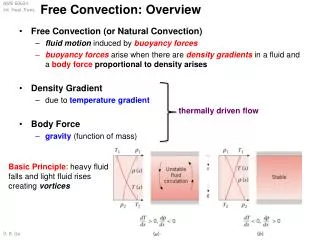
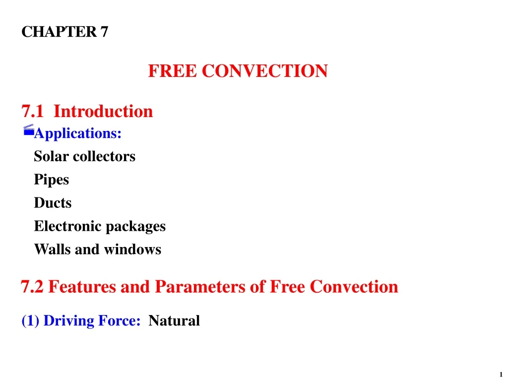
FREE CONVECTION 7.1 Introduction Solar collectors Pipes Ducts Electronic packages Walls and windows 7.2 Features and Parameters of Free Convection (1) Driving Force: Natural 1
Requirements: (i) Acceleration field, (ii) Density gradient (2) Governing Parameters: Two: 2
(5) External vs. Enclosure free convection: (i) External: over: Vertical surfaces Inclined surfaces Horizontal cylinders Spheres (ii) Enclosure: in: 4
Rectangular confines Concentric cylinders Concentric spheres (6)Analytic Solution 7.3 Governing Equations Approximations: (1) Density is constant except in gravity forces 5
(2) Boussinesq approximation: relate density change to temperature change (3) Negligible dissipation Assume: Steady state Two-dimensional Laminar Continuity: x-momentum: 6
y-momentum: Energy: NOTE: (1) Gravity points in the negative x-direction (2) Flow and temperature fields are coupled 7
7.3.1 Boundary Layer Equations • Velocity and temperature boundary layers • Apply approximation used in forced convection y-component of the Navier-Stokes equations reduces to External flow: Neglect ambient pressure variation in x Furthermore, for boundary layer flow 8
x-momentum: Neglect axial conduction Energy: (7.4) becomes 9
7.4 Laminar Free Convection over a Vertical Plate: Uniform Surface Temperature Determine: velocity and temperature distribution 7.4.1 Assumptions • (1) Steady state • Laminar flow • (3) Two-dimensional 10
(1)Constant properties (2)Boussinesq approximation (3)Uniform surface temperature (4)Uniform ambient temperature (5)Vertical plate (9) Negligible dissipation 7.4.2 Governing Equations Continuity: x-momentum: 11
where is a dimensionless temperature defined as Energy: 7.4.3 Boundary Conditions Velocity: 12
Temperature: 7.4.4 Similarity Transformation 13
Stream function satisfies continuity (7.9) into (7.8)7 Local Grashof number: Let 14
Combining (7.5), (7.7), (7.8), (7.12), (7.16), (7.17) NOTE Transformation of boundary conditions: Velocity: 16
NOTE: (1) Three PDE are transformed into two ODE (3) Five BC are needed (4) Seven BC are transformed into five (5) One parameter: Prandtl number. 7.4.5 Solution • (7.18) and (7.19) are solved numerically • Solution is presented graphically • Figs. 7.2 gives u(x,y) • Fig. 7.3 gives T(x,y) 18
7.4.5 Heat Transfer Coefficient and Nusselt Number Start with Use (7.8) and (7.10) 21
Define:local Nusselt number: Average heat transfer coefficient (7.21) into (2.50), integrate Average Nusselt number 22
d d (3) (4) , t Special Cases Example 7.1: Vertical Plate at Uniform Surface Temperature 24
Solution (1) Observations • External free convection • Vertical plate • Uniform surface temperature • Check Rayleigh number for laminar flow (2) Problem Definition 25
Determine flow and heat transfer characteristics for free convection over a vertical flat plate at uniform surface temperature. (3) Solution Plan • Laminar flow? Compute Rayleigh number • If laminar, use Figs. 7.2 and 7.3. • Use solution for Nu and h (4) Plan Execution (i) Assumptions • Newtonian fluid • Steady state • Boussinesq approximations • Two-dimensional 26
(6) Flat plate (7) Uniform surface temperature (8) No dissipation (9) No radiation. (ii) Analysis and Computation Compute the Rayleigh number: 27
Substituting into (7.2) Thus the flow is laminar (1) Axial velocity u: 29
Solve for u (1) Temperature T: 31
Solve for 32
(5) Local Nusselt number: Nusselt Number: Use (7.22), evaluate at x = L = 0.08 m 33
(6) Local heat transfer coefficient: at x = L = 0.08 m (7) Heat flux: Newton’s law gives (8) Total heat transfer: 34
(iii) Checking Dimensional check: Quantitative check: 35
Infinite fluid at temperature (5) Comments 7.5 Laminar Free Convection over a Vertical Plate: Uniform Surface Heat Flux • Vertical Plate • Uniform surface heat flux • Assumptions: Same as Section 7.4 36
Governing equations: Same as Section 7.4 • Boundary conditions: Replace uniform surface temperature with • uniform surface flux • Solution: Similarity transformation (Appendix F) • Results: (1) Surface temperature 37
Example 7.2: Vertical Plate at Uniform Surface Flux (1) Surface temperature (2) Nusselt number (3) Heat transfer coefficient Solution (1) Observations • External free convection • Vertical plate 39
Uniform surface heat flux • Check Rayleigh number for laminar flow • If laminar: (2) Problem Definition (3) Solution Plan • Laminar flow? Compute Rayleigh number 40
(4) Plan Execution (i) Assumptions (10) Newtonian fluid (11) Steady state (12) Boussinesq approximations (13) Two-dimensional (15) Flat plate 41
(16) Uniform surface heat flux (17) No dissipation (18) No radiation (ii) Analysis Rayleigh number: Surface temperature: Nusselt number: 42
Heat transfer coefficient (iii) Computations 43
Substitute into (7.2) • Flow is laminar 46
Result: 47
Thus, 48
Use (d)-(f) to tabulate results at x = 0.02, 0.04, 0.06 and 0.08 m (iii) Checking 50