Objective
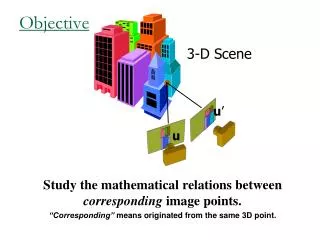
Objective. 3-D Scene. u ’. u. Study the mathematical relations between corresponding image points. “Corresponding” means originated from the same 3D point. Two-views geometry Outline . Background: Camera, Projection models Necessary tools: A taste of projective geometry

Objective
E N D
Presentation Transcript
Objective 3-D Scene u’ u Study the mathematical relations between corresponding image points. “Corresponding”means originated from the same 3D point.
Two-views geometryOutline • Background: Camera, Projection models • Necessary tools: A taste of projective geometry • Two view geometry: • Planar scene (homography ). • Non-planar scene (epipolar geometry). • 3D reconstruction (stereo).
Perspective Projection • Origin (0,0,0)is the Focal center • X,Y (x,y) axis are along the image axis (height / width). • Z is depth = distance along the Optical axis • f – Focal length
Coordinates in Projective Plane P2 Take R3 –{0,0,0} and look at scale equivalence class (rays/lines trough the origin). k(0,1,1) k(1,1,1) “Ideal point” k(0,0,1) k(1,0,1) k(x,y,0)
2D Projective Geometry: Basics • A point: • A line: we denote a line with a 3-vector • Line coordinates are homogenous • Points and lines are dual: p is on l if • Intersection of two lines/points
Cross Product in matrix notation [ ]x Hartley & Zisserman p. 581
2D Projective Transformation • H is defined up to scale • 9 parameters • 8 degrees of freedom • Determined by 4 corresponding points how does H operate on lines? Hartley & Zisserman p. 32
Two-views geometryOutline • Background: Camera, Projection • Necessary tools: A taste of projective geometry • Two view geometry: • Homography • Epipolar geometry, the essential matrix • Camera calibration, the fundamental matrix • 3D reconstruction from two views (Stereo algorithms)
Two View Geometry • When a camera changes position and orientation, the scene moves rigidly relative to the camera 3-D Scene u’ u Rotation + translation
Two View Geometry (simple cases) • In two cases this results in homography: • Camera rotates around its focal point • The scene is planar Then: • Point correspondence forms 1:1mapping • depth cannot be recovered
Camera Rotation (R is 3x3 non-singular)
Planar Scenes Scene • Intuitively A sequence of two perspectivities • Algebraically Need to show: Camera 2 Camera 1
Summary: Two Views Related by Homography Two images are related by homography: • One to one mapping from p to p’ • H contains 8 degrees of freedom • Given correspondences, each point determines 2 equations • 4 points are required to recover H • Depth cannot be recovered
The General Case: Epipolar Lines epipolar line
Epipolar Plane P epipolar plane epipolar line epipolar line O O’ Baseline
Epipole • Every plane through the baseline is an epipolar plane • It determines a pair of epipolar lines (one in each image) • Two systems of epipolar lines are obtained • Each system intersects in a point, the epipole • The epipole is the projection of the center of the other camera epipolar plane epipolar lines epipolar lines O’ O Baseline
Epipolar Lines To define an epipolar plane, we define the plane through the two camera centers O and O’ and some point P. This can be written algebraically (in some world coordinates as follows: P epipolar plane epipolar line epipolar line O O’ Baseline
Essential Matrix (algebraic constraint between corresponding image points) • Set world coordinates around the first camera • What to do with O’P? Every rotation changes the observed coordinate in the second image • We need to de-rotate to make the second image plane parallel to the first • Replacing by image points Other derivations Hartley & Zisserman p. 241
Essential Matrix (cont.) • Denote this by: • Then • Define • E is called the “essential matrix”
Properties of the Essential Matrix • E is homogeneous • Its (right and left) null spaces are the two epipoles • 9 parameters • Is linear E, • E can be recovered up to scale using 8 points. • Has rank 2. • The constraint detE=0 7 points suffices • In fact, there are only 5 degrees of freedom in E, • 3 for rotation • 2 for translation (up to scale), determined by epipole
Camera Internal Parameters or Calibration matrix • Background The lens optical axis does not coincide with the sensor • We model this using a 3x3 matrix the Calibration matrix
Camera Calibration matrix • The difference between ideal sensor ant the real one is modeled by a 3x3 matrix K: • (cx,cy) camera center, (ax,ay) pixel dimensions, b skew • We end with
Fundamental Matrix • F, is the fundamental matrix.
Properties of the Fundamental Matrix • F is homogeneous • Its (right and left) null spaces are the two epipoles • 9 parameters • Is linear F, • F can be recovered up to scale using 8 points. • Has rank 2. • The constraint detF=0 7 points suffices
Epipolar Plane P l x X’ l’ e’ e O O’ Baseline Other derivations Hartley & Zisserman p. 223
Stereo Vision • Objective: 3D reconstruction • Input: 2 (or more) images taken with calibrated cameras • Output: 3D structure of scene • Steps: • Rectification • Matching • Depth estimation
Rectification • Image Reprojection • reproject image planes onto common plane parallel to baseline • Notice, only focal point of camera really matters (Seitz)
Rectification • Any stereo pair can be rectified by rotating and scaling the two image planes (=homography) • We will assume images have been rectified so • Image planes of cameras are parallel. • Focal points are at same height. • Focal lengths same. • Then, epipolar lines fall along the horizontal scan lines of the images
Cyclopean Coordinates • Origin at midpoint between camera centers • Axes parallel to those of the two (rectified) cameras
Disparity • The difference is called “disparity” • dis inversely related to Z: greater sensitivity to nearby points • dis directly related to b: sensitivity to small baseline
Main Step: Correspondence Search • What to match? • Objects? More identifiable, but difficult to compute • Pixels? Easier to handle, but maybe ambiguous • Edges? • Collections of pixels (regions)?
Random Dot Stereogram • Using random dot pairs Julesz showed that recognition is not needed for stereo
1D Search • More efficient • Fewer false matches SSD error disparity
Comparison of Stereo Algorithms D. Scharstein and R. Szeliski. "A Taxonomy and Evaluation of Dense Two-Frame Stereo Correspondence Algorithms," International Journal of Computer Vision,47 (2002), pp. 7-42. Scene Ground truth
Results with window correlation Window-based matching (best window size) Ground truth
Graph Cuts (next class). Graph cuts Ground truth