Download
1 / 26
391 likes | 853 Views
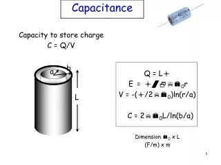
Chapter 6. Dielectrics and Capacitance. Capacitance of a Two-Wire Line. The configuration of the two-wire line consists of two parallel conducting cylinders, each of circular cross section.

E N D
Chapter 6 Dielectrics and Capacitance Capacitance of a Two-Wire Line • The configuration of the two-wire line consists of two parallel conducting cylinders, each of circular cross section. • We shall be able to find complete information about the electric field intensity, the potential field, the surface charge density distribution, and the capacitance. • This arrangement is an important type of transmission line.
Chapter 6 Dielectrics and Capacitance Capacitance of a Two-Wire Line • The potential field of two infinite line charges, with a positive line charge in the xz plane at x = a and a negative line at x = –a, is shown below. • The potential of a single line charge with zero reference at a radius of R0 is: • The combined potential field can be written as:
Chapter 6 Dielectrics and Capacitance Capacitance of a Two-Wire Line • We choose R10 = R20, thus placing the zero reference at equal distances from each line. • Expressing R1 and R2 in terms of x and y, • To recognize the equipotential surfaces, some algebraic manipulations are necessary. • Choosing an equipotential surface V = V1, we define a dimensionless parameter K1 as:
Chapter 6 Dielectrics and Capacitance Capacitance of a Two-Wire Line • After some multiplications and algebra, we obtain: • The last equation shows that the V = V1 equipotential surface is independent of z and intersects the xz plane in a circle of radius b, • The center of the circle is x = h, y = 0, where:
Chapter 6 Dielectrics and Capacitance Capacitance of a Two-Wire Line • Let us now consider a zero-potential conducting plane located at x = 0, and a conducting cylinder of radius b and potential V0 with its axis located a distance h from the plane. • Solving the last two equations for a and K1 in terms of b and h, • The potential of the cylinder is V0, so that: • Therefore,
Chapter 6 Dielectrics and Capacitance Capacitance of a Two-Wire Line • Given h, b, and V0, we may determine a, K1, and ρL. • The capacitance between the cylinder and the plane is now available. For a length L in the z direction, • Prove the equity by solving quadratic equation in eα, where cosh(α)=h/b.
Chapter 6 Dielectrics and Capacitance Capacitance of a Two-Wire Line • Example • The black circle shows the cross section of a cylinder of 5 m radius at a potential of 100 V in free space. Its axis is 13 m away from a plane at zero potential.
Chapter 6 Dielectrics and Capacitance Capacitance of a Two-Wire Line • We may also identify the cylinder representing the 50 V equipotential surface by finding new values for K1, b, and h.
Chapter 6 Dielectrics and Capacitance Capacitance of a Two-Wire Line
Chapter 6 Dielectrics and Capacitance - - - - - - - - + + + + + + + + Capacitance of a Two-Wire Line
Chapter 6 Dielectrics and Capacitance Capacitance of a Two-Wire Line • For the case of a conductor with b << h, then:
Chapter 6 Dielectrics and Capacitance Capacitance of a Two-Wire Line • For the case of a conductor with b << h, then:
Engineering Electromagnetics Chapter 8 The Steady Magnetic Field
Chapter 8 The Steady Magnetic Field The Steady Magnetic Field • At this point, we shall begin our study of the magnetic field with a definition of the magnetic field itself and show how it arises from a current distribution. • The relation of the steady magnetic field to its source is more complicated than is the relation of the electrostatic field to its source. • The source of the steady magnetic field may be a permanent magnet, an electric field changing linearly with time, or a direct current. • Our present concern will be the magnetic field produced by a differential dc element in the free space.
Chapter 8 The Steady Magnetic Field Biot-Savart Law • Consider a differential current element as a vanishingly small section of a current-carrying filamentary conductor. • We assume a current I flowing in a differential vector length of the filament dL. • The law of Biot-Savart then states that • “At any point P the magnitude of the magnetic field intensity produced by the differential element is proportional to the product of the current, the magnitude of the differential length, and the sine of the angle lying between the filament and a line connecting the filament to the point P at which the field is desired; also, the magnitude of the magnetic field intensity is inversely proportional to the square of the distance from the differential element to the point P.”
Chapter 8 The Steady Magnetic Field Biot-Savart Law • The Biot-Savart law may be written concisely using vector notation as • The units of the magnetic field intensity H are evidently amperes per meter (A/m). • Using additional subscripts to indicate the point to which each of the quantities refers,
Chapter 8 The Steady Magnetic Field Biot-Savart Law • It is impossible to check experimentally the law of Biot-Savart as expressed previously, because the differential current element cannot be isolated. • It follows that only the integral form of the Biot-Savart law can be verified experimentally,
Chapter 8 The Steady Magnetic Field Biot-Savart Law • The Biot-Savart law may also be expressed in terms of distributed sources, such as current density J (A/m2) and surface current density K (A/m). • Surface current flows in a sheet of vanishingly small thickness, and the sheet’s current density J is therefore infinite. • Surface current density K, however, is measured in amperes per meter width. Thus, if the surface current density is uniform, the total currentIin any width b is where the width b is measured perpendicularly to the direction in which the current is flowing.
Chapter 8 The Steady Magnetic Field Biot-Savart Law • For a nonuniform surface current density, integration is necessary: where dNis a differential element of the path across which the current is flowing. • Thus, the differential current element IdL may be expressed in terms of surface current density K or current density J, and alternate forms of the Biot-Savart law can be obtained as and
Chapter 8 The Steady Magnetic Field Biot-Savart Law • We may illustrate the application of the Biot-Savart law by considering an infinitely long straight filament. • Referring to the next figure, we should recognize the symmetry of this field. As we moves along the filament, no variation of z or occur. • The field point r is given by r = ρaρ, and the source point r’ is given by r’ = z’az. Therefore,
Chapter 8 The Steady Magnetic Field Biot-Savart Law • We take dL = dz’az and the current is directed toward the increasing values of z’. Thus we have • The resulting magnetic field intensity is directed to aφdirection.
Chapter 8 The Steady Magnetic Field Biot-Savart Law • Continuing the integration with respect to z’ only, • The magnitude of the field is not a function of φ or z. • It varies inversely with the distance from the filament. • The direction of the magnetic-field-intensity vector is circumferential.
Chapter 8 The Steady Magnetic Field Biot-Savart Law • The formula to calculate the magnetic field intensity caused by a finite-length current element can be readily used: • Try to derive this formula
Chapter 8 The Steady Magnetic Field Biot-Savart Law • Example • Determine H at P2(0.4,0.3,0) in the field of an 8 A filamentary current directed inward from infinity to the origin on the positive x axis, and then outward to infinity along the y axis. • What if the line goes onward to infinity along the z axis?
Chapter 8 The Steady Magnetic Field Homework 9 • D6.6. • D8.1. • D8.2. • Deadline: 03.07.2012, at 08:00.