Download
1 / 45
490 likes | 854 Views
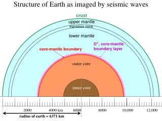
Structure of Earth as imaged by seismic waves. crust. upper mantle. transition zone. lower mantle. D”, core-mantle boundary layer. core-mantle boundary. outer core. inner core. 2000. 4000 km. 6000. 8000. 10,000. 12,000. radius of earth = 6371 km.

E N D
Structure of Earth as imaged by seismic waves crust upper mantle transition zone lower mantle D”, core-mantle boundary layer core-mantle boundary outer core inner core 2000 4000 km 6000 8000 10,000 12,000 radius of earth = 6371 km
Seismic waves involve stress, strain, and density • Two important types of stresses and strains: • Pressure, P and volume change per unit volume, DV/V • Shear stress and shear strain
For linear elasticity, Hooke’s law applies: stress = elastic_constant x strain
For elastic waves, two elastic constants are key: And density of the material, r r = mass/volume
Two types of elastic waves Compressional or P waves • involve volume change and shear Shear or S waves • involve only shear Click on these links to see particle motions: P wave particle motions S wave particle motions
Elastic wave velocities determined by material properties P wave velocity S wave velocity
epicenter Earth surface ray perpendicular to wavefront expanding wavefront at some instant of time after earthquake occurrence seismograph station Earth center
epicenter tt(D) = total travel time along ray from earthquake to station Earth surface ray D = epicentral distance in degrees D seismograph station Earth center
Globally recorded earthquakes during the past 40 years earthquake depth 0-33 km 33-70 70-300 300-700
2,538,185 travel time observations from International Seismological Centre (ISC), for earthquakes with depths between “0” and 60 km. time, minutes These are the commonly reported phases as reported to the ISC from seismograph stations from around the world; see phase types on next page distance, degrees
click on link to P and S phases in the earth PKPPKP PPS SSS PPP PS SS PKKP SKKS water waves surface waves PKS SKS PKP PPP PKIKP S PP ScS diffracted P PcS PcP These lines represent plus or minus one minute errors in reading arrival times P
Nomenclature for seismic body phases P wave segments in blue S wave segments in red Por S mantle K outer core I or J inner core i = reflection at inner core-outer core boundary c = reflection at core mantle boundary
Single path refracted through mantle S P seismic wave source Inner core Outer core Mantle
2,538,185 travel time observations from International Seismological Centre (ISC), for earthquakes with depths between “0” and 60 km. time, minutes S P diffracted around core P These are the commonly reported phases as reported to the ISC from seismograph stations from around the world; see phase types on next page distance, degrees
Single reflection at surface PP SS Inner core Outer core Mantle
2,538,185 travel time observations from International Seismological Centre (ISC), for earthquakes with depths between “0” and 60 km. SS time, minutes PP These are the commonly reported phases as reported to the ISC from seismograph stations from around the world; see phase types on next page distance, degrees
Single reflection at core-mantle boundary PcP reflection
2,538,185 travel time observations from International Seismological Centre (ISC), for earthquakes with depths between “0” and 60 km. time, minutes ScS PcS PcP These are the commonly reported phases as reported to the ISC from seismograph stations from around the world; see phase types on next page distance, degrees
P in mantle, refracting to P in the outer core (K) and out through the mantle as P PKP P K P
P segments in mantle, P segments in outer core (K), and P segment in inner core (I) PKIKP P K I K P
2,538,185 travel time observations from International Seismological Centre (ISC), for earthquakes with depths between “0” and 60 km. time, minutes PKP PKIKP These are the commonly reported phases as reported to the ISC from seismograph stations from around the world; see phase types on next page distance, degrees
S in mantle, refracting and converting to P in outer core, then refracting back out and converting back to S in the mantle SKS S K S
S in mantle, refracting and converting to P in outer core, P reflects once at inner side of core-mantle boundary, then refracting back out back with conversion to S in the mantle SKKS S reflection K K S
2,538,185 travel time observations from International Seismological Centre (ISC), for earthquakes with depths between “0” and 60 km. time, minutes SKKS SKS S These are the commonly reported phases as reported to the ISC from seismograph stations from around the world; see phase types on next page distance, degrees
Compressional (P) and Shear (S) wave velocities, Vp and Vs seismic wave velocity km/sec upper mantle depth transition zone km lower mantle D’’ layer outer core inner core
For self compression of homogeneous material f (R) = k/r k = - dP/(dV/V) = dP/(dr/r) dP = - g r dR where R = radius to a point in the earth, and g = gravitational acceleration at that radius g = GMR/R2 where MR = mass within sphere of radius R dr/dR = -f/rg
For self compression of homogeneous material dr/dR = -f/rg • This is the gradient in density determined by the seismic wave velocities. To obtain density, one must integrate by fixing the density, r, and gravity, g, at the top of the layer and calculating both r and g as one proceeds downwards. • The calculation assumes • a simple compression of material that does not change chemistry or phase. • the compression as one goes deeper produces an adiabatic temperature increase.
For self compression of homogeneous material dr/dR = -f/rg • The method is applied to the following layers: • upper mantle • lower mantle • outer core • inner core To determine the jumps in density between these layers, the following constraints are used: Mass of earth Moment of Inertia of Earth Periods of free oscillations of Earth
Density, r kg/m3 km core-mantle boundary depth, km
Gravitational acceleration, g m/s2 km core-mantle boundary depth, km
Pressure, P GPa. km core-mantle boundary depth, km
Density vrs pressure kg/m3 GPa.
Density vrs pressure Inner core/outer core boundary core-mantle boundary kg/m3 compression liquid to solid composition change phase changes compression mantle density crustal density GPa.
chemical stratification and differentiation basaltic-granitic crust phase changes Mg(Fe) silicates fluid, 90% iron solidified iron 2000 4000 km 6000 8000 10,000 12,000
Earth’s convective systems cool, strong lithospheric boundary layer crust slowly convecting mantle: plate tectonic engine seafloor spreading core-mantle thermo-chemical boundary layer subduction rapidly convecting outer core: geomagnetic dynamo solid inner core 2000 4000 km 6000 8000 10,000 12,000
Temperature in mantle Temperature, degrees C 0 2000 3000 4000 5000 1000 near surface thermal boundary layer = lithosphere conductive heat flow upper mantle transition zone mantle melting mantle convection advective heat flow Adiabatic gradient lower mantle Adiabatic gradient D” = Lower mantle thermo-chemical boundary layer D” conductive heat flow ? CMB iron melting outer core
Mantle convection, hot spots and plumes Lowrie, Fundamentals of Geophysics, Fig. 6.26
abstract Average P-wave velocity perturbation in the lowermost 1000 km of the mantle
crust Generation of Earth’s magnetic field in the outer core mantle outer core • The geomagnetic dynamo: • turbulent fluid convection • electrically conducting fluid • fluid flow-electromagnetic interactions • effects of rotation of earth inner core 2000 4000 km 6000 8000 10,000 12,000