Download

1 / 22
220 likes | 334 Views
Welfare and Profit Maximization with Production Costs. A. Blum, A. Gupta, Y. Mansour , A. Sharma. Model. Multiple buyers Arbitrary valuation Multiple products Mechanism: prices Online setting Goals: Maximize Welfare Maximize Profit. Main Focus: Production cost increases. MODEL.

E N D
Welfare and Profit Maximization with Production Costs A. Blum, A. Gupta, Y. Mansour, A. Sharma
Model • Multiple buyers • Arbitrary valuation • Multiple products • Mechanism: prices • Online setting • Goals: • Maximize Welfare • Maximize Profit Main Focus: • Production cost • increases
MODEL 25₪ 5₪ 7 ₪ 9₪ 21₪ payment SW
cost 25₪ 6₪ 9₪ 9₪ 33₪
Production Cost • CS literature • Unlimited supply • Fixed production cost • Limited Supply • Phase transition • Two extreme alternatives
Production cost: ECON 101 • Increasing marginal production cost S D
This Work • non-decreasing production cost • Posted prices • Online setting $1.99
Our Results: Welfare Maximization • SW = value - cost • Simple algorithm • Price the kthitem of product j by the cost of the (2k)thitem of product j • Constant competitive ratio in many cases • Linear • Polynomial • Logarithmic • Fails for limited supply
Our Results: Welfare Maximization • SW = value - cost • Convex production cost: • Logarithmic competitive ratio • Handles limited supply • [BGN]
Our results: Profit Maximization • Profit = revenue - cost • Logarithmic competitive ratio • Combining: • Social Welfare maximization, multiple buyers • Revenue Maximization, single buyer • Similar to [AAM]
General Structural Theorem • Fix a pricing scheme π • Consider a product prices cost prices opt Items sold Alg profit
General Structural Theorem • Fix a pricing scheme π • Sum the area across products • If ΣjBLUE< αΣjBROWN+ β • Then SW(alg) > (SW(opt)- β)/ α
General Structural Theorem • PROOF • Buyer b buys Sb in π and Ob in opt. • Consider prices πbwhen buyer comes • At the prices of πb : vb (Sb) – πb (Sb) ≥ vb(Ob) – πb (Ob) • Summing over buyers Σbvb (Sb) – πb(Sb) ≥ Σbvb(Ob) – πb(Ob) SW(alg) + C(alg) - P(alg) ≥ SW(opt) + C(opt) - P(opt)
General Structural Theorem • P(alg) - C(alg) = profit(alg) • Maximize the Regret term P(opt) - C(λ) • Fix prices πb to be final prices • Only increases P(opt) • NOW: the term P(opt) - C(λ) = ΣiΣj P(j) – Ci(j) is exactly the sum of the BLUEareas
Twice the index algorithm • For each item j, • The price of k-th copy is cost(2k) • NOTE: increasing cost implies price ≥ cost • Technically Need to compare BLUE vsBROWN Linear Cost: prices cost
Twice the index algorithm • For each item j, • The price of k-th copy is cost(2k) • NOTE: increasing cost implies price > cost • Technically Need to compare BLUE vsBROWN Performance: • Linear cost: c(x)=ax+b α = 1/6β = Σjcj(2)-cj(1) • Polynomial cost c(x)=axd α = 1/2d β = 2(d+2)d+1Σjcj(2) • Logarithmic cost c(x)=ln(x+1) α = ln(3/2)/2 β = 3|J|
Twice the index algorithm • When does it fail?! • Limited supply: • k items with fixed cost • Pricing: • First k/2 at cost • Last k/2 infinite • Very poor SW • Good SW: [BGN] prices cost
Convex Functions • Multiple discrete prices • Enough items for in each price level • Run limited supply per price level • E.g., [BGN] • Smooth shifts between the price levels. • Limit the jump • Assume a given upper bound on values • Umax in [Z/ε, Z]
Convex Functions • Two types of items • Many copies sold • The last completely sold price interval gives the required performance • Few items sold • More problematic • Introduces additive loss • Uses the convexity THEOREM: B=O(log(mn)) C= cost of first B items SW(alg) < [SW(opt) – C]/B
Profit Maximization • Given: • SW maximization algo. A • Approx. ratio α1 , β1 • Single buyer profit max algo. B • Approx ratio α2 , β2 • Output: Profit Max Algorithm • Approx ratio O(α1 α2) , O(β1/(α1 α2)+(mβ2)/α1) • Similar to [AAM]
Profit Maximization • Algorithm • With prob ½ use the prices of A. • If A gets high revenue we are done • With prob. ½ use sum of prices of A and B • B is memoryless (works for a single buyer) • If A gets high revenue we are done • Otherwise: there is a significant welfare left • A maximizes the SW • So B can get a fraction of the remaining SW.
Conclusion • Changing cost of production • Interpolates between the extreme • Well studied in Economics • Reasonable competitive ratio • Constant for many interesting cases • Simple pricing algorithms • Future work: • Offline, better ratios • Decreasing prices, initial results • Beyond convex cost