Download
1 / 21
210 likes | 347 Views
1. Comparison of HOM, SPLIDHOM and INTERP 2. Ideas for the daily benchmark dataset (temperature). Christine Gruber, Ingeborg Auer. Intercomparison experiments. Comparison of: Della-Marta and Wanner, 2006 (HOM) Mestre et al., ???? (SPLIDHOM)

E N D
1. Comparison of HOM, SPLIDHOM and INTERP2. Ideas for the daily benchmark dataset (temperature) Christine Gruber, Ingeborg Auer
Intercomparison experiments • Comparison of: • Della-Marta and Wanner, 2006 (HOM) • Mestre et al., ???? (SPLIDHOM) • Vincent et al., 2002; Brunetti et al., 2006 (INTERP) • I. Semi-synthetic data • Use of parallel measurements • Combination of series: artificial but realistic breaks the truth is known for evaluation of the methods • II. (Preliminary) Application of the methods to a test dataset (Lower Austria) • Uncertainty estimation using bootstrap temperature dependent adjustments
Semi-synthetic data • Parallel measurement breaks • Realistic inhomogeneities (relocation, screen change,..) • Not only temperature dependence included • Can be combined at given break point known position • In Austria not enough stations with long parallel measurements available…
Results for 5 Stations, TMIN/TMAX, 4 seasons=40 series • Absolute differences of percentiles • Homogenized-truth • RAW-truth
Benefit of the homogenization Q10 Q50 Q90 Q10 Q50 Q90 Q10 Q50 Q90 TMIN TMAX SPLIDHOM INTERP HOM
Conclusions • For evaluation parallel measurement data is used + realistic breaks • only 40 time series homogenized (*20 different samples) • Many time series too small inhomogeneities, less temperature dependence • HOM and SPLIDHOM • similar, main differences for extreme values • Improvement of HOM/SPLIDHOM compared to INTERP, in the case that: • Highly correlated reference stations available • Inhomogeneity is temperature dependent
Lower Austria- Experiment • Preliminary analysis of the Lower Austria temperatures • Mainly to see how the methods work for real data • Influence of reference stations, magnitude of the breaks,… • Testing a bootstrap approach for estimating uncertainties • Break detection with HOCLIS and PRODIGE (annual means) • Homogenization with SPLIDHOM (HOM)
WIE summer, SPLIDHOM adjustment [°C] Ref=WMA 1993 1980 1971 1953 temperature [°C] Ref=KRM Ref=HOH Influence of undetected breakpoints (higher order moments) in REF? Too short HSPs for KRM, WMA!
Adjustments Vienna SPLIDHOM Error growth!!!? How many values are required that breaks can be adjusted reliably? Comparison of different methods useful HOM 1993 1980 1971 Uncertainty of the adjustments seems to be reduced for earlier breaks Introduction of a “model” easier to adjust in the following (earlier) breaks
WIE winter SPLIDHOM Ref=KRM Ref=HOH Ref=WMA
WIE (ref=HOH) Q90 Q10 All data estimate Mean of bootstrap sample 0.9 confidence interval Original Annual mean Uncertainties in extremes of the adjustments have hardly any influence (in this case)
WIE (ref=KRM) Q90 Q10 All data estimate Mean of bootstrap sample 0.9 confidence interval Original Annual mean
WIE (ref=WMA) Q90 Q10 All data estimate Mean of bootstrap sample 0.9 confidence interval Original Annual mean
Example for usefulness of uncertainty estimates Q10 No effect of the adjustments on the 0.1 percentile But information about the (minimum) uncertainty of the time series
Example for usefulness of uncertainty estimates Annual mean
Open questions • Requirements for reference stations? • correlation • length of HSPs • Detection of “higher order moment”- breaks? • Is it possible to adjust higher order moments? • Problems due to micro-scale climate changes (test-reference station distribution change) • Uncertainty assessment (especially for extreme values) • method uncertainty • sampling uncertainty • representativeness (references)
The nature of the problem • Extreme value studies homogenization of daily data necessary • Adjusting inhomogeneities in dependence of the weather type, physical reasons (primary effect) • Adjustments as function of wind, sunshine duration, global radiation… (difficult due to data availability) • Adjustment of the temperature dependence of the inhomogeneities (secondary effect) • Adjusting the temperature distribution (e.g. Della-Marta and Wanner, 2006) • Effect of inhomogeneities on temperature percentiles/extremes is reduced (that’s what we want in extreme value studies) In a first step: Shall we take into account only temperature dependent breaks in the daily benchmark?
Significance of temperature dependence How often significant temperature dependence occurs? Typical pattern and range of the magnitude pattern for synthetic inhomogeneities
Possible working steps • Case study • Real dataset, metadata (availability?) • Classification of inhomogeneities due to their source • Examination of temperature dependence? (e.g. HOM) • Other dependencies (wind, radiation,…) • Typical pattern benchmark • Semi-synthetic (parallel measurement) series • Realistic inhomogeneities, but truth is known for evaluation • Dependencies to other elements could be studied (wind, radiation?) • Data availability? (too few stations in Austria) • Surrogate • Based on typical inhomogeneity pattern (temperature dependent) • (If other dependencies shall be treated as well benchmark multiple series???? ( new adjustment-method multi-parameter???) Typical pattern? We must learn more about the problem