
Deep Learning
E N D
Presentation Transcript
Deep Learning Disclaimer: This PPT is modified based on Dr. Hung-yi Lee http://speech.ee.ntu.edu.tw/~tlkagk/courses_ML17.html
Deep learning attracts lots of attention. • I believe you have seen lots of exciting results before. Deep learning trends at Google. Source: SIGMOD 2016/Jeff Dean
Ups and downs of Deep Learning • 1958: Perceptron (linear model) • 1969: Perceptron has limitation • 1980s: Multi-layer perceptron • Do not have significant difference from DNN today • 1986: Backpropagation • Usually more than 3 hidden layers is not helpful • 1989: 1 hidden layer is “good enough”, why deep? • 2006: RBM (Restricted Boltzmann Machines) initialization • 2009: GPU (graphical processing unit) • 2011: Start to be popular in speech recognition • 2012: win ILSVRC image competition • 2015.2: Image recognition surpassing human-level performance • 2016.3: Alpha GO beats Lee Sedol • 2016.10: Speech recognition system as good as humans
https://pdfs.semanticscholar.org/presentation/c139/cf0377dddf95d8a268652dd9c51631279400.pdfhttps://pdfs.semanticscholar.org/presentation/c139/cf0377dddf95d8a268652dd9c51631279400.pdf
https://pdfs.semanticscholar.org/presentation/c139/cf0377dddf95d8a268652dd9c51631279400.pdfhttps://pdfs.semanticscholar.org/presentation/c139/cf0377dddf95d8a268652dd9c51631279400.pdf
https://pdfs.semanticscholar.org/presentation/c139/cf0377dddf95d8a268652dd9c51631279400.pdfhttps://pdfs.semanticscholar.org/presentation/c139/cf0377dddf95d8a268652dd9c51631279400.pdf
https://pdfs.semanticscholar.org/presentation/c139/cf0377dddf95d8a268652dd9c51631279400.pdfhttps://pdfs.semanticscholar.org/presentation/c139/cf0377dddf95d8a268652dd9c51631279400.pdf
Introduction to deep learning • Dr. XiaogangWang: • Check out PPT: page 5-28 http://www.ee.cuhk.edu.hk/~xgwang/deep_learning_isba.pdf https://www.enlitic.com/?fbclid=IwAR3H3RRnw_BK756MJt-l34C3w4QgVMZfcf8cDrPaxBxajo-oRxJh6nEnUoc https://automatedinsights.com/customer-stories/associated-press/?fbclid=IwAR0H8Pq-o-bbTFcTff8hS6fz0hO1osIvOS-e3pZC66y9Zn7s-Ok0iWJ7Q5c
Three Steps for Deep Learning Neural Network Deep Learning is so simple ……
Neural Network “Neuron” Neural Network Different connection leads to different network structures Network parameter :all the weights and biases in the “neurons”
Fully Connect Feedforward Network 0.98 4 1 1 -2 1 0.12 -1 -2 -1 1 0 Sigmoid Function
Fully Connect Feedforward Network 0.98 0.62 4 0.86 2 3 1 1 -1 -1 -2 0 2 -2 1 0 0 0.12 -2 -1 -1 0.83 -2 0.11 -1 -1 4 1
Fully Connect Feedforward Network 0.72 0.51 0.73 2 3 1 0 -1 -1 -2 -2 0 1 0.5 -2 -1 -1 0.85 0.12 0 -1 4 1 0 2 0 This is a function. Input vector, output vector Given network structure, define a function set
Fully Connect Feedforward Network neuron Layer 1 Layer 2 Layer L Input Output y1 …… …… y2 …… …… …… …… …… …… yM Output Layer Input Layer Hidden Layers
Deep = Many hidden layers 22 layers http://cs231n.stanford.edu/slides/winter1516_lecture8.pdf 19 layers 8 layers 6.7% 7.3% 16.4% AlexNet (2012) GoogleNet (2014) VGG (2014)
Deep = Many hidden layers 101 layers 152 layers Special structure Ref: https://www.youtube.com/watch?v=dxB6299gpvI 3.57% 7.3% 6.7% 16.4% GoogleNet (2014) Residual Net (2015) VGG (2014) AlexNet (2012) Taipei 101
Matrix Operation 0.98 4 1 1 -2 1 0.12 -1 -2 -1 1 0
Review: Example 0.98 0.62 4 0.86 2 3 1 1 -1 -1 -2 -2 2 1 0 0 0 0.12 -2 -1 -1 0.83 -2 0.11 -1 -1 4 1 Q: Completely write out the Matrix Operation for this fully Connect Feedforward Network.
Neural Network y1 …… W1 WL W2 y2 …… bL b2 b1 …… …… …… …… …… x a1 y a2 …… yM x a1 bL b2 b1 W1 W2 WL + + + aL-1
Neural Network y1 …… W1 WL W2 y2 …… bL b2 b1 …… …… …… …… …… x a1 y a2 …… yM Using parallel computing techniques to speed up matrix operation y x x bL b1 b2 W1 WL W2 … … + + +
Matryoshkadoll https://en.wikipedia.org/wiki/Matryoshka_doll
Output Layer as Multi-Class Classifier Feature extractor replacing feature engineering y1 …… …… y2 …… …… …… Softmax …… …… …… yM Input Layer = Multi-class Classifier Output Layer Hidden Layers The last fully-connected layer is called the “output layer”. For classification, it represents the class scores.
Example Application Input Output y1 y2 is 1 0.1 …… is 2 0.7 The image is “2” y10 …… …… 0.2 is 0 16 x 16 = 256 Each dimension represents the confidence of a digit. Ink → 1 No ink → 0
Example Application • Handwriting Digit Recognition y1 is 1 y2 Machine is 2 …… Neural Network “2” …… …… y10 is 0 What is needed is a function …… Input: 256-dim vector output: 10-dim vector
Example Application Input Layer 1 Layer 2 Layer L Output y1 …… is 1 y2 …… A function set containing the candidates for Handwriting Digit Recognition is 2 “2” …… …… …… …… …… …… y10 …… is 0 Output Layer Input Layer Hidden Layers You need to decide the network structure to let a good function in your function set.
FAQ • Q: How many layers? How many neurons for each layer? • Q: Can the structure be automatically determined? • E.g. Evolutionary Artificial Neural Networks • Q: Can we design the network structure? + Intuition Trial and Error Convolutional Neural Network (CNN)
Three Steps for Deep Learning Neural Network Deep Learning is so simple ……
Loss for an Example target “1” …… 1 y1 …… 0 Given a set of parameters y2 Softmax …… …… …… …… …… Cross Entropy …… …… y10 0
Total Loss Total Loss: For all training data … NN Find a function in function set that minimizes total loss L NN yN xN y1 y2 y3 x1 x2 x3 NN …… …… …… …… Find the network parameters that minimize total loss L NN
Three Steps for Deep Learning Neural Network Deep Learning is so simple ……
Gradient Descent Compute 0.2 0.15 Compute -0.1 0.05 …… Compute 0.3 0.2 gradient ……
Gradient Descent Compute Compute 0.2 0.15 0.09 …… Compute Compute -0.1 0.05 0.15 …… …… Compute Compute 0.3 0.2 0.10 …… ……
Gradient Descent This is the “learning” of machines in deep learning …… Even alpha go using this approach. People image …… Actually ….. I hope you are not too disappointed :p
Backpropagation • Backpropagation: an efficient way to compute in neural network libdnn 台大周伯威 同學開發 • Ref: http://speech.ee.ntu.edu.tw/~tlkagk/courses/MLDS_2015_2/Lecture/DNN%20backprop.ecm.mp4/index.html
Three Steps for Deep Learning Neural Network Deep Learning is so simple ……