Introductory NMR 101
Chemical Shift. Introductory NMR 101. Chemical Shift. Peak Intensity. Spin-spin Coupling. Sample Preparation: Deuterated Solvents. Spin-spin Coupling. Karplus (Garbisch) Relationships: Correlation of Magnitude of J Value w/ Geometry. 14 12 10 8 6 4 2 0.

Introductory NMR 101
E N D
Presentation Transcript
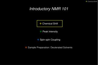
Chemical Shift Introductory NMR 101 Chemical Shift Peak Intensity Spin-spin Coupling Sample Preparation: Deuterated Solvents
Spin-spin Coupling Karplus (Garbisch) Relationships: Correlation of Magnitude of J Value w/ Geometry 14 12 10 8 6 4 2 0
Spin-spin Coupling Protocola-c for Computational/NMR Strategy 1. Determine as many experimental coupling constants Jexp( 3J and 4J) as possible. 2. Subject each diastereomer to multiconformational search (e.g., Monte Carlo in MacroModel) to identify the family of stable conformational isomers and then compute the Boltzmann weighted coupling constants Jcalc for each diastereomer. Calculate 2’between the experimental Js and the computed Js. The isomer with smallest 2’ (best fit) is the proposed structure. 2’ = ∑(Jexp-Jcalc)2
Spin-spin Coupling Extracting Coupling Constants from First Order Multiplets • 4096J. Org. Chem.1994,59, 4096-4103 • A Practical Guide to First-Order Multiplet Analysis in • 1H NMR Spectroscopy • Thomas R. Hoye,* Paul R. Hanson,1a and James R. Vyvyan1b • Department of Chemistry, University of Minnesota, Minneapolis, Minnesota 55455 • Received March 11, 1994 • The ability to deduce the proper set of coupling constant (J) values from a complex first-order multiplet in a 1H NMR spectrum is an extremely important asset. This is particularly valuable to the task of assigning relative configurations among two or more stereocenters in a molecule. Most books and treatises that deal with coupling constant analysis address the less useful operation of generating splitting trees to create the line pattern from a given set of J values. Presented here are general and systematic protocols for the converse--i.e., for deducing the complete set of J values from the multiplet. Two analytical methods (A. systematic analysis of line spacings and B. construction of what can be called inverted splitting trees) are presented first. A reasonably thorough and systematic set of graphical representations of common doublet of doublets (dd's), ddd's, and dddd's are then presented. These constitute a complementary method for identification of J's through visual pattern recognition. These approaches are effective strategies for extraction of coupling constant values from even the most complex first-order multiplets.
Spin-spin Coupling Extracting Coupling Constants from NMR Multiplets: An Addendum H H "A Practical Guide to First-Order Multiplet Analysis in 1H NMR Spectroscopy," Hoye, T. R.; Hanson, P. R.; Vyvyan, J. R. J. Org. Chem.1994, 59, 4096-4103. "A Method for Easily Determining Coupling Constants. An Addendum to …" Hoye, T. R.; Zhao, H. J. Org. Chem.2002, 67, 4014-4016.
Spin-spin Coupling Two Steps to Identify all J’s in a Multiplet 1. Assign each peak in the multiplet one or more component numbers from 1 to 2n (arbitrarily) from left to right by analogy to the examples shown below.
Spin-spin Coupling 2. Systematically identify the J's by the following series of steps. Adopt the convention that J1 ≤ J2 ≤ J3 ≤ J4 ≤ … Jn. Appreciate that for J3 and beyond it is necessary to have first determined the previous coupling constants (e.g., both J1 and J2 must be known before J3 can be determined). {1 to x} is the distance in Hz between component 1 (i.e., the lefthandmost peak) and component x. i) {1 to 2} is J1 ii) {1 to 3} is J2 iii) remove from further consideration the component corresponding to (J1 + J2) iv) {1 to next higher remaining component (i.e., 4 or 5)} is J3 corollary: one of {1 to 4} or {1 to 5} is J3 v) remove from further consideration the components corresponding to the remaining combinations of the first three J values [i.e., (J1 + J3), (J2 + J3), and (J1 + J2 + J3) vi) {1 to the next higher remaining component} is J4 corollary: one of {1 to 5} through {1 to 9} is J4
Spin-spin Coupling Application to a dddd (24 = 16)
Spin-spin Coupling Application to a dddd (24 = 16)
Spin-spin Coupling 2. Systematically identify the J's by the following series of steps. Adopt the convention that J1 ≤ J2 ≤ J3 ≤ J4 ≤ … Jn. Appreciate that for J3 and beyond it is necessary to have first determined the previous coupling constants (e.g., both J1 and J2 must be known before J3 can be determined). {1 to x} is the distance in Hz between component 1 (i.e., the lefthandmost peak) and component x. i) {1 to 2} is J1 ii) {1 to 3} is J2 iii) remove from further consideration the component corresponding to (J1 + J2) iv) {1 to next higher remaining component (i.e., 4 or 5)} is J3 corollary: one of {1 to 4} or {1 to 5} is J3 v) remove from further consideration the components corresponding to the remaining combinations of the first three J values [i.e., (J1 + J3), (J2 + J3), and (J1 + J2 + J3) vi) {1 to the next higher remaining component} is J4 corollary: one of {1 to 5} through {1 to 9} is J4
Spin-spin Coupling Application to a dddd (24 = 16)
Spin-spin Coupling Assigning Component #’s is Harder for Some Multiplets (e.g., dddddd)
Spin-spin Coupling Resolution Enhancement: Relative Line Intensity Now Easier 6 8 3 3 5 3 2 1 1
Spin-spin Coupling Splitting Tree: to Confirm the Assignments
Spin-spin Coupling Spiruchostatins A and B: A Challenging Opportunity to Test the Method
Spin-spin Coupling Strategies for Ferreting Out the Js • To overcome peak broadening: • a) Variable temperature NMR • b) Resolution enhancement • To overcome peak overlap: • Mixed solvents: benzene-d6 “titration” • Complementary field strengths
Spin-spin Coupling Variable Temperature NMR 60 °C 25 °C
Spin-spin Coupling Resolution Enhancement Gives Critical 3’’’-H (ddddd) Js For easy deconvolution of first order Js see: Hoye, T. R.; Zhao, H. J. Org. Chem. 2002, 67, 4014-4016. 60 °C
Spin-spin Coupling Resolution Enhancement (cont’d)
Spin-spin Coupling Overcome Peak Overlap by Mixed Solvent( 17 % Benzene-d6 in CDCl3) 17 % C6D6 60 °C 0 % C6D6