Brute-Force Triangulation
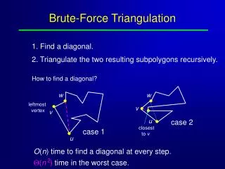
w. v. w. v. 2. ( n ) time in the worst case. . u. u. Brute-Force Triangulation . 1. Find a diagonal. 2. Triangulate the two resulting subpolygons recursively. How to find a diagonal?. leftmost vertex. case 2. closest to v. case 1.

Brute-Force Triangulation
E N D
Presentation Transcript
w v w v 2 (n )time in the worst case. u u Brute-Force Triangulation 1. Find a diagonal. 2. Triangulate the two resulting subpolygons recursively. How to find a diagonal? leftmost vertex case 2 closest to v case 1 O(n) time to find a diagonal at every step.
Triangulating a Convex Polygon (n)time! Idea: monotone Decompose a simple polygon into convex pieces. Triangulate the pieces. as difficult as triangulation
y-monotone Pieces y-axis y-monotone if any line perpendicular to the y-axis has a connected intersection with the polygon. highest vertex Stragegy: walk always downward or horizontal Partition the polygon into monotone pieces and then triangulate. lowest vertex
Turn Vertex Turn vertex is where the walk from highest vertex to the lowest vertex switches direction. At vertex v Both adjacent edges are below. v The polygon interior lies above. Choose a diagonal that goes up.
q p q p Merge vetex: lies below its two neighbors and has interior angle > . Split vetex: lies above its two neighbors and has interior angle > . End vetex: lies below its two neighbors and has interior angle < . Start vetex: lies above its two neighbors and has interior angle < . Regular vetex: the remaining vertices (no turn). Five Types of Vertices Point p = (x, y) is “below” a different point q = (u, v) if y < v or y = v and x > u. Otherwise p is “above” q. 4 types of turn vertices What happens if we rotate the polygon by ? start vertices end vertices split vertices merge vertices start vertices end vertices
Proof Suppose the polygon is not y-monotone. We prove that it contains a split or merge vertex. exterior l q p interior interior p = r q l r p r= p exterior Local Non-Monotonicity Lemma A polygon is y-monotone if it has no split or merge vertices. split vertex There exists a horizontal line l intersecting the polygon in >1 components, of which the leftmost is a segment between some vertices p (left) and q (right). Start at q, traverse the boundary counterclockwise until it crosses the line l again at point r. r Traverse in the oppose direction from q and crosses line l again at point r’. The lowest point during this traversal must be a merge vertex. r The highest vertex during the traversal from q to r must be a split vertex. merge vertex
The next event found in time O(log n). Partitioning into Monotone Pieces The lemma implies that the polygon will have y-monotone pieces once its split and merge vertices are removed. Add a downward diagonal at every merge vertex. Add an upward diagonal at every split vertex. Use a downward plane sweep. No new event point will be created except the vertices. The event queue is implemented as priority queue (e.g., heap).
v : split vertex i e : edge immediately to its left. j e : edge immediately to its right. k h(e ) i h(e ): lowest vertex above v and between e and e . i i j k or the upper vertex of e if such vertex does not exist. j e e e e v j i-1 i i k Connect v to h(e ). i i Removal of a Split Vertex edge helper
Merge vertices can be handled the same way in an upward sweep as split vertices in a downward sweep. v : highest vertex below the sweep line and between e and e . v : merge vertex i m But why not all in the same sweep? e : edge immediately to its left. j e : edge immediately to its right. k j k Connect v to v . m In case the helper of e is not replaced any more, connect to its lower endpoint. v will replace v as the helper of e . Check if the old helper is a merge vertex and add the diagonal if so. (The diagonal is always added if the new helper is a split vertex). m i j v v e e i i k m j j Removal of a Merge Vertex
Only edges to the left of the polygon interior are stored. Edges are stored in the left-to-right order. With every edge e its helper h(e) is also stored. Sweep-Line Status Implemented as a binary search tree. This is because we are only interested in edges to the leftof split and merge vertices.
Construct a doubly-connected edge list to represent the polygon. Add in diagonals computed for split and merge vertices. Edges in the status BST and corresponding ones in DCEL cross-point each other. DCEL Representation n vertices + n edges + 2 faces (initially) Adding an edge can be done in O(1) time.
The Algorithm MakeMonotone(P) Input: A simple polygon P stored in DCEL D. Output: A partitioning of P into monotone subpolygons stored in D. 1. Q priority queue storing vertices of P 2. T // initialize the status as a binary search tree. 3. i 0 4. while Q 5. do v the highest priority vertex from Q// removal from Q 6. case v of 7. start vertex: HandleStartVertex(v ) 8. end vertex: HandleEndVertex(v ) 9. split vertex: HandleSplitVertx(v ) 10. merge vertex: HandleMergeVertex(v ) 11. regular vertex: HandleRegularVertex(v ) 12. i i + 1 i i i i i i i
HandleStartVertex(v ) 1. T T { e } 2. h(e ) v // set the helper i i i i • HandleEndVertex(v ) • ifh(e ) is a merge vertex • then insert the diagonal • connecting v to h(e ) • in D • 3. T T – { e } i i –1 i i –1 i -1 v e v v v v e v v v v v v v e e e e v e e e v e e v e e e e 11 11 13 14 1 2 4 4 7 8 10 12 15 3 9 9 8 6 7 5 5 6 2 3 12 14 15 1 13 10 Handling Start & End Vertices insert into T
HandleSplitVertex(v ) • Search in T to find e directly left of v • insert the diagonal connect v to h(e ) • into D • h(e ) v • 4. T T + { e } • 5. h(e ) v i j i i j j i i i i v v v e v v v v v v e v v v v e e e e e v e e e e e v e e e 15 6 7 9 13 9 11 11 12 12 4 1 10 4 5 3 14 2 13 2 5 7 1 8 6 3 10 15 8 14 Handling Split Vertex
j i • HandleMergeVertex(v ) • ifh(e ) is a merge vertex • then insert the diagonal • connecting v to h(e ) • in D • 3. T T – { e } • Search in T to find the edge e • directly left of v . • 5. ifh(e ) is a merge vertex • then insert the diagonal • connecting v to h(e ) • in D • 6. h(e ) v j i i –1 i j i i –1 j i i -1 v v v e v v v v v e v v v v e v e e e v e v e e e e e e e e 9 13 15 14 1 2 4 4 7 8 10 11 3 12 11 10 8 6 7 5 5 6 1 13 3 15 2 14 12 9 Handling Merge Vertex (1)
h(e ) j j i • HandleMergeVertex(v ) • ifh(e ) is a merge vertex • then insert the diagonal • connecting v to h(e ) • in D • 3. T T – { e } • Search in T to find the edge e • directly left of v . • 5. ifh(e ) is a merge vertex • then insert the diagonal • connecting v to h(e ) • in D • 6. h(e ) v j i i –1 i j i i –1 j i i -1 v e e i – 1 i j Handling Merge Vertex (2) h(e ) i –1
HandleRegularVertex(v ) • if the polygon interior lies to the right • of v • 2. then ifh(e ) is a merge vertex • 3. then insert the diagonal • connecting v to h(e ) • in D • 4. T T – { e } • 5. T T + { e } • 6. h(e ) v • 7. else search in T to find the edge e • directly left of v . • 8. ifh(e ) is a merge vertex • then insert the diagonal • connecting v to h(e ) • in D • 9. h(e ) v i i i –1 i i –1 i -1 i i i j i j i j i v v v v v v v v e v v v v e v e v e e e e v e e e e e e e e j 14 15 1 2 3 6 4 11 8 10 9 13 4 11 5 9 10 8 6 7 5 12 7 1 15 13 2 3 14 12 Handling Regular Vertices (1)
HandleRegularVertex(v ) • if the polygon interior lies to the right • of v • 2. then ifh(e ) is a merge vertex • 3. then insert the diagonal • connecting v to h(e ) • in D • 4. T T – { e } • 5. T T + { e } • 6. h(e ) v • 7. else search in T to find the edge e • directly left of v . • 8. ifh(e ) is a merge vertex • then insert the diagonal • connecting v to h(e ) • in D • 9. h(e ) v i i i –1 i i –1 h(e ) j i -1 i i i j i j i j i v e j i j Handling Regular Vertices (2)
Correctness Theorem The algorithm adds a set of non-intersecting diagonals that partitions the polygon into monotone pieces. Proof The pieces that result from the partitioning contain no split or merge vertices. Hence they are monotone by an earlier lemma. We need only prove that the added segments are diagonals that intersect neither the polygon edges nor each other. Establish the above claim for the handling of each of the five type of vertices during the sweep. (Read the textbook on how to do this for the case of a split vertex.)
Running Time on Partitioning MakeMonotone(P) Input: A simple polygon P stored in DCEL D. Output: A partitioning of P into monotone subpolygons stored in D. 1. Q priority queue storing vertices of P 2. T 3. i 0 4. whileQ 5. dov the highest priority vertex from Q 6. case vof 7. start vertex: HandleStartVertex(v ) 8. end vertex: HandleEndVertex(v ) 9. split vertex: HandleSplitVertx(v ) 10. merge vertex: HandleMergeVertex(v ) 11. regular vertex: HanleRegularVertex(v ) 12. i i + 1 // O(n) // O(log n) i i // O(log n) each case i // queries and updates // in O(log n) time and // insertion of a diagonal // in O(1) time. i i i i Total time: O(n log n) Total storage: O(n)
One boundary of the funnel is a polygon edge. The other boundary is a chain of reflex vertices (with interior angles > ) plus one convex vertex (the highest) at bottom of the stack. Triangulating a y-Monotone Polygon Assumption The polygon is strictly y-monotone (no horizontal edges). It is for clarity of presentation and will be easily removed later. Order of processing: in decreasing y-coordinate. A stack S: vertices that have been encountered and may still need diagonals. convex vertex lowest vertex on top. funnel Idea: add as many diagonals from the current vertex handled to those on the stack as possible. current vertex Invariants of iteration: reflex vertices
Push the previous top of the stack and the current vertex back onto the stack. Pop these vertices from the stack. Add diagonals from the current vertex to them (except the bottom one) as they are popped. u u u u u u u u u u u j –3 j –3 j –4 j –2 j –4 j –2 j –1 j –1 j j –1 j Case 1: Next Vertex on Opposite Chain This vertex must be the lower endpoint of the single edge e bounding the chain. e current vertex
Pop one vertex from the stack. It shares an edge with the current vertex. Pushed the last popped vertex back onto the stack followed by the current vertex. Pop other vertices from the stack as long as they are visible from the current vertex. Draw a diagonal between each of them and the current vertex. u u u u u u u u u u u u u u j –3 j j –1 j –4 j –2 j –3 j –2 j –5 j –4 j –1 j j –5 j –5 j –4 Case 2: Next Vertex on the Same Chain The vertices that can connect to the current vertex are all on the stack. current vertex
The Triangulation Algorithm • TriangulateMonotonePolygon(P) • Input: A strictly y-monotone polygon P stored in DCEL D. • Output: A triangulation of P stored in D. • Merge the vertices on the left and right chains into one sequence • sorted in decreasing y-coordinate. (In case there is a tie, the one • with smaller x-coordinate comes first.) • 2. Push(u , S) • Push(u , S) • forj 3 ton – 1 • do ifu and Top(S) are on different chains • then while Next(Top(S)) NULL • v Top(S) • Pop(S) • insert a diagonal from u to v • Pop(S) • Push(u , S) • Push(u , S) • else Pop(S) • while Top(S) is visible from u inside the polygon • v Top(S) • insert a diagonal between u and v • Push(v, S) • Push(u , S) 1 2 j j j –1 j j j j
u u u u u u u u u u u u u u u u u 2 2 5 5 1 5 4 1 1 1 3 6 2 1 3 2 4 u u u u u u u u u u u u u u u u u u u u 14 17 18 13 16 6 20 15 11 9 12 19 8 7 1 4 5 2 3 10 An Example Start: j =4: j =3: j =5: j =6:
u u u u u u u u u u u u u u u u u 8 8 10 10 6 7 9 7 6 8 7 9 11 6 8 5 10 u u u u u u u u u u u u u u u u u u u u 9 14 13 11 10 15 16 20 12 6 7 4 5 8 3 2 1 17 19 18 Example (cont’d) j = 7: j =9: j =8: (result) j =10: j =11:
u u u u u u u u u u u u u u u u 10 10 18 19 17 18 17 17 15 16 17 10 10 16 15 15 u u u u u u u u u u u u u u u u u u u u 10 17 9 1 6 19 13 3 14 12 7 15 11 16 2 18 5 20 8 4 Example (Cont’d) j = 15: j = 16: j = 17: (result) j = 18: j = 19:
#pushes 2n - 4 #pops #pushes Treat them from left to right. The effect of this is equivalent to that of rotating the plane slightly clockwise and then every vertex will have different y coordinate. Removal of Strict y-monotonicity The running time of TriangulateMonotonePolygon is(n). What to do if some vertices have the same y-coordinates?
Time Complexity of Triangulation 1. Partition a simple polygon into monotone pieces. O(n log n) 2. Triangulate each monotone piece. (n) for all monotone pieces together Theorem A simple polygon can be triangulated in O(n log n) time and O(n) storage.
The plane sweep for decomposition of a polygon into monotone pieces takes as input only edges that lie to the left of the interior. This easily generalizes to a planar subdivision in a bounding box. Triangulation of a Planar Subdivision The algorithm for splitting a polygon into monotone pieces does not use the fact that the polygon was simple. Thus a planar subdivision with n vertices can also be triangulated in O(n log n) time using O(n) storage.