Thermospheric Variability MCDP Work
Paul Withers withers@bu.edu Boston University MAVEN PSG, Berkeley CA 2011.10.19-20. Thermospheric Variability MCDP Work. But first… Mariner 9 radio occultation electron density profiles. ~100 found at NSSDC Extend to ~400km Ionopause height (Unlike MGS) Spans immense dust storm

Thermospheric Variability MCDP Work
E N D
Presentation Transcript
Paul Withers withers@bu.edu Boston University MAVEN PSG, Berkeley CA 2011.10.19-20 Thermospheric VariabilityMCDP Work
But first… Mariner 9 radio occultation electron density profiles ~100 found at NSSDC Extend to ~400km Ionopause height (Unlike MGS) Spans immense dust storm Better geographical and SZA coverage than MGS Anyone want digital copies of these ~100 profiles?
What's the weather like at 150 km? • Climate = What you expect (predictions from models) • Weather = What you get (less predictable from numerical models) • Operations need predictions of both • I'm working on some data products associated with empirical measurements of thermospheric variability
Aerobraking accelerometers • MGS, ODY, MRO sampled range of seasons, locations, times of day, solar cycle, etc • Density profiles, as well as density scale heights • Pressure proportional to density x scale height These four profiles should be identical
MGS RS ionospheric data • 5600 profiles of electron density vs altitude • Altitude of peak occurs at predictable pressure level • Width of peak indicates neutral temperature Longitude
Task 1 (Intrinsic variability) • Variability at same Ls, latitude, longitude, LST, altitude (everything but day-to-day) • Occurs for aerobraking when period x N = sol Numbers are standard deviation of selected density measurements relative to mean
Task 1 – Accelerometer results • MGS, ODY, MRO • Inbound and outbound • Dayside and nightside • 100 km to 160 km in 10 km intervals • Density, density scale height, pressure(-ish)
MRO Outbound 130 km Nightside Density Numbers are standard deviation of selected density measurements relative to mean
MRO Outbound 130 km Nightside Scale Height
MRO Outbound 130 km Nightside Pressure
Task 1 – Radio science results • MGS • Mars Years 24, 25, 26, and 27 • Variations in peak altitude and fitted scale height • Also peak altitude changes normalized by scale height (can be used to get sense of variations in pressure at fixed altitude)
2.5 degree latitude spacing 20 degree longitude spacing 1 hour LST spacing 15 degree Ls spacing Need 7 points in a 4-D box to define a cluster
Standard deviation of: Difference between main peak altitude and a cluster’s main peak altitude, divided by the average scale height for that cluster Typical values are 0.2
Task 2 (Variations with longitude) • Longitude has a surprisingly large effect on thermospheric densities and temperatures • Report standard deviation of density, etc, at fixed Ls, latitude, LST, altitude • Identify conditions where thermal tides are strong
Task 2 – Radio science results • Similar sort of approach, using variations in peak altitude and fitted scale height • Select Mars Year (e.g. 27) and latitude range (e.g. 60N to 70N) • Find that selected subset of data forms groups with narrow range in Ls (~15-30 deg) and LST (1-2 hrs) • Look at variations with longitude for each group
Task 3 (Response to extreme solar events) – not yet started • Solar flares • CMEs • Responses not well-known, may be small and hard to measure • May be large at times Densities at 150 km increase during period of high solar EUV flux
Task 4 (Response to dust storms) MGS TES dust opacity Noachis dust storm during aerobraking MGS Accelerometer density at 140 km outbound during dust storm
Where’s the dust? Orbit 25, Ls = 203 Orbit 51, Ls = 227 Orbit 53, Ls = 228-ish Inbound data at 50N Outbound data at 30N Storm at 50S
Decay timescale is longer closer to the storm Dust opacity itself decays faster closer to the storm - ? Decay timescale in degrees of Ls
Next steps on this Task • ODY aerobraking started in waning phase of a dust storm • Some MGS radio occultation data (>60N) likely to encompass dust storm conditions
Conclusions • Tasks 1 and 2 (basic statistics of variability) completed, but deliverables are gigantic set of tables/figures without much interpretation • Task 4 (dust storm) well underway, results so far are operationally and scientifically interesting • Task 3 (extreme solar events) will be started soon