Transform and Conquer: Analysis and Design of Algorithms - Unit III, Chapter 6
Learn about the transform-and-conquer technique in algorithm analysis and design, including presorting, balanced search trees, AVL trees, 2-3 trees, and heaps and heapsort.
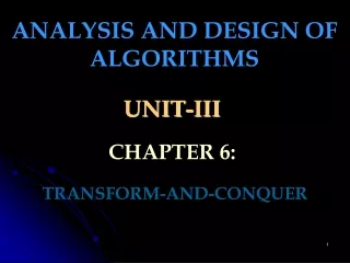

Transform and Conquer: Analysis and Design of Algorithms - Unit III, Chapter 6
E N D
Presentation Transcript
ANALYSIS AND DESIGN OF ALGORITHMS UNIT-III CHAPTER 6: TRANSFORM-AND-CONQUER
OUTLINE • Presorting • Balanced Search Trees • AVL Trees • 2-3 Trees • Heaps and Heapsort
Introduction Transform-and-conquer technique These methods work as two-stage procedures. (1) Transformation stage: the problem’s instance is modified to be, for one reason or another, more amenable to solution. (2) In the conquering stage, it is solved.
Transform and Conquer This group of techniques solves a problem by a transformation to a simpler/more convenient instance of the same problem. We call it instance simplification. to a different representation of the same instance. We call it representation change. to a different problem for which an algorithm is already available. We call it problem reduction. Figure:Transform-and-conquer strategy.
Instance simplification - Presorting Solve a problem’s instance by transforming it into another simpler/easier instance of the same problem Presorting: Many problems involving lists are easier when list is sorted. searching checking if all elements are distinct (element uniqueness) Also: Topological sorting helps solving some problems for dags. Presorting is used in many geometric algorithms.
Element Uniqueness with presorting Presorting-based algorithm Stage 1: sort by efficient sorting algorithm (e.g. merge sort). Stage 2: scan array to check pairs of adjacent elements. Efficiency: T(n) = Tsort(n) + Tscan(n) ЄΘ(nlog n) + Θ(n) = Θ(nlog n) Brute force algorithm Compare all pairs of elementsEfficiency:Θ(n2)
Example 1Checking element uniqueness in an array. ALGORITHM PresortElementUniqueness(A[0..n - 1]) //Solves the element uniqueness problem by sorting the array first //Input: An array A[0..n - 1] of orderable elements //Output: Returns “true” if A has no equal elements, “false” otherwise Sort the array A for i 0 to n - 2 do if A[i]= A[i + 1] return false return true • We can sort the array first and then check only its consecutive elements: if the array has equal elements, a pair of them must be next to each other and vice versa.
Example 2Computing a mode • A mode is a value that occurs most often in a given list of numbers. For example, for 5, 1, 5, 7, 6, 5, 7, the mode is 5. • The brute-force approach for computing a mode would scan the list and compute the frequencies of all its distinct values, then find the value with the largest frequency. • To implement this, we can store the values already encountered, along with their frequencies, in a separate list. • On each iteration, the ith element of the original list is compared with the values already encountered by traversing this auxiliary list. • If a matching value is found, its frequency is incremented; otherwise, the current element is added to the list of distinct values with a frequency of 1.
Example 2Computing a mode • Since list’s ith element is compared with i – 1 elements of the auxiliary list of distinct values seen so far before being added to the list with a frequency of 1, the worst-case number of comparisons made by this algorithm in creating the frequency list is n C(n) = ∑ (i-1) = 0 + 1 + . . . + (n-1) = (n-1)n ЄΘ(n2). i=1 2 The additional n – 1 comparisons are needed to find the largest frequency in the auxiliary list. • In presort mode computation algorithm, the list is sorted first. Then all equal values will be adjacent to each other. To compute the mode, all we need to do is to find the longest run of adjacent equal values in the sorted array. • The efficiency of this presort algorithm will be nlogn, which is the time spent on sorting.
Example 2Computing a mode ALGORITHM PresortMode(A[0..n - 1]) //Computes the mode of an array by sorting it first //Input: An array A[0..n - 1] of orderable elements //Output: The array’s mode Sort the array A i 0 //current run begins at position i modefrequency ← 0 //highest frequency seen so far while i ≤ n – 1 do runlength ← 1; runvalue ← A[i] while i + runlength ≤ n – 1 and A[i + runlength] = runvalue runlength ← runlength + 1 ifrunlength > modefrequency modefrequency ← runlength; modevalue ← runvalue i ← i + runlength returnmodevalue
Example 3: Searching Problem Problem: Search for a given K in A[0..n-1] Presorting-based algorithm: Stage 1 Sort the array by an efficient sorting algorithm. Stage 2 Apply binary search. Efficiency: T(n) = Tsort(n) + Tsearch(n) = Θ(nlog n) + Θ(log n) = Θ(nlog n)
Binary Trees • Binary Tree: A binary tree is a finite set of elements that is either empty or is partitioned into three disjoint subsets: - The first subset contains a single element called the ROOT of the tree. - The other two subsets are themselves binary trees, called the LEFT and RIGHT subtrees of the original tree. • NODE : Each element of a binary tree is called a node of the tree.
A B E C D F Left subtree Right subtree BINARY TREE Note: A node in a binary tree can have no more than two subtrees.
BINARY SEARCH TREE Binary Search Tree (Binary Sorted Tree) : • Suppose T is a binary tree. Then T is called a binary search tree if each node of the tree has the following property : the value of each node is greater than every value in the left subtree of that node and is less than every value in the right subtree of N. • Let x be a node in a binary search tree . If y is a node in the left subtree of x,then info(y)<info(x). If y is a node in the right subtree of x , then info(x)<=info(y) x All≥x All<x
Example BSTs: 2 5 3 3 7 7 2 4 8 5 8 4
Draw the BSTs of height 2, 3, 4, 5, 6 on the following set of keys: { 1, 4, 5, 10, 16, 17, 21 } 17 16 16 21 10 17 10 10 4 17 4 21 4 1 5 16 21 1 5 1 5 HEIGHT 2 HEIGHT 3 HEIGHT 4 21 17 1 21 17 16 21 4 17 16 10 5 16 10 5 10 or or 10 5 4 16 4 4 17 1 1 5 1 21 HEIGHT 6 HEIGHT 5
Operations of BSTs: Insert • Adds an element x to the tree so that the binary search tree property continues to hold • The basic algorithm • set the Index to Root • Check if the data where index is pointing is NULL, if so Insert x in place of NULL, and finish the process. • If the data is not NULL then compare the data with inserting item • If the inserting item is equal or bigger then traverse to the right else traverse to the left. • Continue with 2nd step again until
Insert Operations: 1st of 3 steps • The function begins at the root node and compares item 32 with the root value 25. Since 32 > 25, we traverse the right • subtree and look at node 35.
Insert Operations: 2nd of 3 steps 2) Considering 35 to be the root of its own subtree, we compare item 32 with 35 and traverse the left subtree of 35.
Insert Operations: 3rd of 3 steps • Create a leaf node with data value 32. Insert the new node as • the left child of node 35.
Insert in BST Insert Key 52. Start at root. 52 > 51 Go right. 51 14 72 06 33 53 97 43 13 99 25 64 84
Insert Key 52. Insert in BST 52 > 51 Go right. 51 14 72 06 33 53 97 43 13 99 25 64 84
Insert Key 52. Insert in BST 51 14 72 52 < 72 Go left. 06 33 53 97 43 13 99 25 64 84
Insert Key 52. Insert in BST 51 14 72 52 < 72 Go left. 06 33 53 97 43 13 99 25 64 84
Insert Key 52. Insert in BST 51 14 72 06 33 53 97 52 < 53 Go left. 43 13 99 25 64 84
Insert Key 52. 52 Insert in BST 51 14 72 No more tree here. INSERT HERE 06 33 53 97 52 < 53 Go left. 43 13 99 25 64 84
Operations of BSTs: Search • looks for an element x within the tree • The basic algorithm • Set the index to root • Compare the searching item with the data at index • If (the searching item is smaller) then traverse to the left else traverse to the right. • Repeat the process until the index is point to NULL or found the item.
Search in BST Search for Key 43. 51 14 72 06 33 53 97 43 13 99 25 64 84
Search in BST Search for Key 43. Start at root. 51 43 < 51 Go left. 14 72 06 33 53 97 43 13 99 25 64 84
Search in BST Search for Key 43. 43 < 51 Go left. 51 14 72 06 33 53 97 43 13 99 25 64 84
Search in BST Search for Key 43. 51 14 72 43 > 14 Go right. 06 33 53 97 43 13 99 25 64 84
Search in BST Search for Key 43. 51 14 72 43 > 14 Go right. 06 33 53 97 43 13 99 25 64 84
Search in BST Search for Key 43. 51 14 72 06 33 53 97 43 > 33 Go right. 43 13 99 25 64 84
Search in BST Search for Key 43. 51 14 72 06 33 53 97 43 > 33 Go right. 43 13 99 25 64 84
Search in BST Search for Key 43. 51 14 72 06 33 53 97 43 13 99 25 64 84 43 = 43 FOUND
Search in BST Search for Key 52. Start at root. 52 > 51 Go right. 51 14 72 06 33 53 97 43 13 99 25 64 84
Search in BST Search for Key 52. 52 > 51 Go right. 51 14 72 06 33 53 97 43 13 99 25 64 84
Search in BST Search for Key 52. 51 14 72 52 < 72 Go left. 06 33 53 97 43 13 99 25 64 84
Search in BST Search for Key 52. 51 14 72 52 < 72 Go left. 06 33 53 97 43 13 99 25 64 84
Search in BST Search for Key 52. 51 14 72 06 33 53 97 52 < 53 Go left. 43 13 99 25 64 84
Search in BST Search for Key 52. 51 14 72 06 33 53 97 52 < 53 Go left. 43 13 99 25 64 84 No more tree here. NOTFOUND
DELETION: 70 70 35 75 35 75 20 65 20 65 90 KEY 50 50 70 70 KEY 35 35 90 75 20 65 20 65 90 50 50
Binary Search Trees • The transformation from a set to a binary search tree is an example of the representation-change technique. • By doing this transformation, we gain in the time efficiency of searching, insertion, and deletion, which are all in Θ(log n), but only in the average case. In the worst case, these operations are in Θ(n).
Balanced Search Trees • There are two approaches to balance a search tree: • The first approach is of instance – simplification variety: an unbalanced binary search tree is transformed to a balanced one. An AVL tree requires the difference between the heights of the left and right subtrees of every node never exceed 1. Other types of trees are red-black trees and splay trees. • The second approach is of the representation-change variety: allow more than one element in a node of a search tree. Specific cases of such trees are 2 – 3 trees, 2-3-4 trees, B-trees.
AVL TREES • AVL trees were invented in 1962 by two Russian scientists, G. M. Adelson-Velsky and E. M. Landis, after whom this data structure is named. • Definition: An AVL tree is a binary search tree in which the balance factor of every node, which is defined as the difference between the heights of the node’s left and right subtrees, is either 0, +1 or -1. (The height of the empty tree is defined as -1). 2 1 10 10 0 0 0 1 5 20 5 20 -1 1 -1 1 0 7 4 7 12 4 0 0 0 0 2 8 2 8 (a) (b) Figure: (a) AVL tree. (b) Binary search tree that is not an AVL tree. The number above each node indicates that node’s balance factor.
AVL TREES • If an insertion of a new node makes an AVL tree unbalanced, we transform the tree by a rotation. • A rotation in an AVL tree is a local transformation of its subtree rooted at a node whose balance has become either +2 or -2; if there are several such nodes, we rotate the tree rooted at the unbalanced node that is the closest to the newly inserted leaf. • There are only four types of rotations: • Single right rotation (R-rotation) • Single left rotation (L-rotation) • Double left-right rotation (LR – rotation) • Double right-left rotation (RL – rotation)
AVL TREES • Single right rotation (R-rotation): This rotation is performed after a new key is inserted into the left subtree of the left child of a tree whose root had the balance if +1 before the insertion. (Imagine rotating the edge connecting the root and its left child in the binary tree in below figure to the right.) 0 2 2 3 1 1 3 0 0 2 R 0 1 3 R 0 2 1 (c) Balanced tree (b) Unbalanced tree after inserting 1 (a) Balanced tree
c r single R-rotation r c T3 T1 T2 T2 T3 T1 Figure:General form of the R-rotation in the AVL tree. A shaded node is the last one inserted. • Note: • These tranformations should not only guarantee that a resulting tree is balanced, but they should also preserve the basic requirements of a binary search tree. • For example, in the initial tree in the above figure, all the keys of subtree T1 are smaller than c, which is smaller than all the keys of subtree T2, which are smaller than r, which is smaller than all the keys of subtree T3. • The same relationships among the key values should hold for the balanced tree after rotation.
AVL TREES • Single left rotation (L-rotation): • This is the mirror image of the single R-rotation. • This rotation is performed after a new key is inserted into the right subtree of the right child of a tree whose root had the balance if -1 before the insertion. (Imagine rotating the edge connecting the root and its right child in the binary tree in below figure to the left.) - 2 0 - 1 1 2 1 - 1 L 0 0 0 2 L 1 3 2 0 (c) Balanced tree 3 (b) Unbalanced tree after inserting 3 (a) Balanced tree
AVL TREES • Double left-right rotation (LR-rotation): • It is performed after a new key is inserted into the right subtree of the left child of a tree whose root had the balance of +1 before the insertion. 2 2 3 3 1 - 1 3 1 1 2 0 R 1 0 0 L 1 2 (a) Balanced tree 0 (b) Unbalanced tree after inserting 2 2 0 0 1 3 (c) Balanced tree