Download
1 / 30
300 likes | 447 Views
SAMSI: 2007-08 Program on Random Media. A hybrid approach of large-eddy simulation and immersed boundary method for flapping wings at moderate Reynolds numbers. Guo-wei He Department of Aerospace Engineering, Iowa State University And Institute of Mechanics Chinese Academy of Sciences

E N D
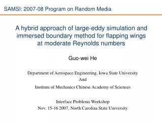
SAMSI: 2007-08 Program on Random Media A hybrid approach of large-eddy simulation and immersed boundary method for flapping wings at moderate Reynolds numbers Guo-wei He Department of Aerospace Engineering, Iowa State University And Institute of Mechanics Chinese Academy of Sciences Interface Problems Workshop Nov. 15-16 2007, North Carolina State University
Objectives and goals • Objectives: • Develop a hybrid approach of LES and IB to simulate plunge and /or pitching motions of an SD7003 airfoil at Re=60k • Investigate the flow field and the aerodynamics performance of an SD7003 airfoil in plunge and/or pitching motions • Goals: • Develop a computational tool to predict the aerodynamics of flapping wing with experimental validation • Provide quantitative documentation of the flow field and the aerodynamics performance of flapping wings by computations LES=Large-eddy simulation, IB=immersed boundary
Free stream T.E. L.E. Cp C/4 C C : chord length; L.E. : leading edge; T.E. : trailing edge; Cp : center of pitching schematical illustration of a SD7003 airfoil A SD7003 airfoil in flapping motion • A low speed airfoil with 8.5% thickness and 1.4% camber • High frequency pitch and/or plunge motion
Laminar-turbulent transition over an SD7003 airfoil • Fixed wings: turbulent transition with separation & reattachment • - The 1st stage: receptivity; - 2: Linear growth stage; • - 3. Nonlinear instabilities stage; - 4. Turbulence transition stage • Flapping wings: compound with turbulence • - Weis-Fogh’s clap and fling; - Leading-edge vortices; • - Pitching-up rotation; - Wake-capture; • The challenges in numerical simulations: • - Laminar-turbulent transition: turbulent flow and its transition • - Plunge and/or pitching airfoil: moving boundary
Large-eddy simulation (LES) for turbulent & transitional flows • LES vs DNS and RANS • Time accurate LES in statistics • LES correctly predicts energy spectra Subgrid scale models are developed on energy budget equation • LES is being developed to predict frequency spectra or time correlations. That is a new challenge. 1. He GW, R. Rubinstein & LP Wang, PoF 14 2186-2193 (2002) 2. He GW, M. Wang & SK Lele, PoF 16 3859-3867 (2004)
LES: a brief introduction Large eddy simulation (LES)velocity =large scales + small scales computed modeled • Filtered Velocity: , G is a filter. The filtered Navier-Stokes equation • Key issues in LES: the filtered N-S equation • Subgrid scale modeling: energy dissipations filter sizes • Numerical algorithm: truncated errors grid sizes • Grid generation • P. Moin, Inter. J. Heat & Fluid flows, 23 (2002) 710-720
LES of an SD 7003 airfoil from Re=10, 000 and 1,000,000 • The number of grid points exceeds the present computer capacity; Most of the points are used to resolve inner layers Wall models needed • Flapping wings: moving boundaries • Grid embedding or multi-domain strategies : increase cost • Unstructured grids: negative impact on stability and convergence • Classic deformation or re-meshing strategies: additional overhead 1. U Piomelli & E. Balaras: Ann. Rev. Fluid Mech. 2002 34:349-74 2. Computer capacity: A Pentium III 933MHz workstation with 1GB of memory
Numerical methods for moving boundaries • Four different IB strategies for complex geometries • A direction forcing at Lagrangian points • Interpolation based on volume of fraction • Explicit linear interpolation • Ghost cell approach
A direct forcing approach (a IB method) • Virtual forces are prescribed on the Cartesian grids to avoid body-fitting grids - represent the effects of body on flows - obtained to impose boundary conditions on body/flow interface • IB for turbulence requires the near wall resolution in all 3 directions • - local refinement • Four essential steps: • - track the locations of body/face interface in a Lagrangian fashion • - formulate an adequate virtual force at the interface locations • - transfer that force smoothly to the Eulerian grid nodes • - time advancement of the Navier-Stokes equations in the Cartesian grids
A hybrid LES and IB method • LES+IB: LES on the Cartesian grids for complex geometries • Challenges: wall modeling on the Cartesian grids - body-fitting: wall modeling in the wall normal direction - Cartesian gird: wall modeling in all three directions
The planned work: wall modeling • A SGS models with a damping function - Damping functions - Eddy viscosity model • Boundary layer equations - wall stress - dynamic models • Shear-dependent SGS models - homogeneous shear flows - wall turbulence
Illustration of IB force Wall treatments in IB/LES method • SGS model: Smagorinsky model • The wall damping function is defined as: • Calculation of : • Minimal distance between Euler grid and Lagrangian point • Calculation of : • Determined from the IB force in the tangent direction
The direct forcing method • Solve the NS equation without forcing for intermediate velocity • Interpolate for Lagrangian velocity • Impose boundary conditions to NS for Lagrangian velocity • Interpolate the force to Eulerian grids • Solve the NS equation with force for Eulerian velocity rsh = pressure + SGS residual stress + viscosity term + convection term
The Navier-Stokes solver • Spatial discretization • Second order finite volume method • Temporal discretization • Fractional step method • Third order Runge-Kutta scheme is used for terms treated explicitly (the convective term and viscosity terms in span-wise direction) • Second order Crank-Nicholson is used for terms treated implicitly (the viscosity terms in stream-wise and cross-wise directions) • Poisson solver • Pre-conditioned conjugate gradient solver
Validation: • The 3D flow around circle cylinders • Body-fitting grids v.s. Cartesian grids • Lift and drag coefficients: vorticity behind cylinders • Turbulent channel flows • Benchmark problem • Mean velocity profile and r.m.s velocity fluctuation
30.0 Shear free Convective BC u=1,v=0,w=0 1.0 10.0 Shear free 5.0 25.0 Validation (I and II): Flow around a circular cylinder Domain size: 30Dx10Dx4D Boundary condition: in-flow: a uniform velocity profile out-flow: a convective boundary condition normal: shear free span-wise: periodic A slice of 3-D Cartesian mesh in z direction Stream and normal directions: the grids stretched to cluster points near surface Span-wise direction: uniform grids
Vortex contour Validation (I): flow around a stationary cylinder Re=100 Stationary Time history of drag and lift coefficients for the flow past an rotating cylinder
Re=200 Angular velocity= Validation (II): flow around a rotating cylinder Time history of drag and lift coefficients for the flow past an rotating cylinder Vortex shedding behind an rotating cylinder
Validation (III): turbulent channel flow using LES and IBM Simulation parameters in x, y, z. • Computation domain: The IB interface is located at y=0.02 • Grid size: in x, y, z. • Reynolds number: based on the wall shear velocity and the channel half-width Mean velocity profile • Boundary condition: y=0.0,non-slip; y=h, non-slip • periodic in x and z directions. • SGS model: dynamic Smagorinsky SGS model • IB method: direct forcing method M. Uhlmann, An immersed boundary method with direct forcing for the simulation of Particulate flows, JCP, 209 (2005) 448-476 R.m.s. velocity fluctuations
Simulation parameters for SD 7003 airfoil • The Reynolds number based on inflow velocity and chord length is : 60,000 • Boundary conditions: • inflow: uniform velocity; outflow: convective boundary condition; • cross wise: shear free; span wise: periodic • Four cases are simulated in present work : • Case1: flow past stationary airfoil SD7003, attack angle= • Case2: flow past plunging airfoil SD7003 • Case3: flow past combined pitching and plunging airfoil • Case4: flow past pitching airfoil SD7003 • Flapping motion:
Simulation parameters: grid setting Two settings of grids are used in present case. • Setting 1 . • Domain size: 60C*60C*0.02C • The center of the airfoil is located at (30C, 30C) • Grid number: 472*332*4 • Mesh size: in the uniform region (IB region): 0.005, the increase proportion is 5% in stream-wise and is 10% in cross-wise, and is uniform in span-wise. • Setting 2. • Domain size: 15C*10C*0.02C • The center of the airfoil is located at (5C, 5C) • Grid number: 570*384*4 • Mesh size: in the uniform region (IB region): 0.005, the increase proportion is 2% in stream-wise,is 4% in cross-wise, and is uniform in span-wise. • Setting 1 is used for all the four cases. Setting 2 is used for case 2 and case 4.
Streamlines and turbulent shear stress for the SD7003 airfoil at Re=60,000, attack angle Case1: stationary • Lift and drag coefficients consistentl with other • author's Q3D results • The transition point is 0.37C from the leading edge • compared with 0.49C (W. Yuan, AIAA, 2005), due to • the poor resolution near the leading edge Lift and drag coefficients for the SD7003 airfoil at Re=60,000
Case1: stationary • The dominant frequency range is from 0.2 to 3 Frequency spectra of the drag coefficient Vortex contour Vortex contour of a stationary airfoil SD7003, attack angle= Frequency spectra of the lift coefficient
Case 2: plunging (frequency=1.25, amplitude=0.05C) • The wake vortex structure shows consistant with experiment’s results. Present case, vortex contour behind trailing edge Expt. From Michael V.OL, AIAA 2007-4233 Dye injection side views for trailing and the near-wake
Case 2: plunging (frequency=1.25, amplitude=0.05C) Vortex contour of a plunging airfoil SD7003, frequency=1.25, amplitude=0.05C
Case 2: plunging (frequency=1, amplitude=0.1C) • The mean Drag Coefficient CD=-0.105, thrust is generated by plunging; • The mean Lift Coefficient CL=0.828 • For drag coefficient, the dominant frequency is f =1,2 • For lift coefficient, the dominant frequency is f =1 Frequency spectra of the drag coefficient Time history of drag and lift coefficients Frequency spectra of the lift coefficient
Case 3: Pitching • The mean drag coefficient CD=0.941 • The mean lift coefficient CL=1.235 • For drag coefficient, the dominant frequency is f=2,4 • For lift coefficient, the dominant frequency is f=2 Frequency spectra of the drag coefficient Time history of drag and lift coefficients Frequency spectra of the lift coefficient
Case 4: combined pitching and plunging motion • The mean drag coefficient CD=0.564 • The mean lift coefficient CL=1.248 • For drag coefficient, the dominant frequency is f =1,2,3,4,5 • For lift coefficient, the dominant frequency is f =1,2 Frequency spectra of the drag coefficient Time history of drag and lift coefficients Frequency spectra of the lift coefficient
Case 4: combined pitching and plunging Vortex contour of a combined pitching and plunging airfoil SD7003
Summary • A hybrid approach of large-eddy simulation and immersed boundary method is developed • Preliminary results for a SD 7003 airfoil at Re=60,000 show the promising of the hybrid approach • Wall models coupled with immersed boundary method need to be developed