Download
1 / 39
390 likes | 423 Views
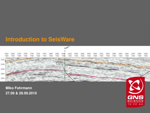
Introduction to SeisWare. Miko Fohrmann 27.09 & 28.09.2010. Goal of the course. The aim of this introductory course in SeisWare is to enable the participants to use the software as a tool for seismic interpretation Note: this is not a ‘ Principles of seismic interpretation’ course!.

E N D
Introduction to SeisWare Miko Fohrmann 27.09 & 28.09.2010
Goal of the course • The aim of this introductory course in SeisWare is to enable the participants to use the software as a tool for seismic interpretation • Note: this is not a ‘Principles of seismic interpretation’ course!
Outline: Monday, 27.09.10 • What are the advantages/disadvantages of SeisWare? • Installation of SeisWare • Launch window – basic structure • Setting up the license server (dongle vs. floating license) • Project setup • Data loading (seismic-, well-, and culture data) • Attaching/copying new data into an existing project • Basemap settings • Displaying seismic lines • Seismic viewer • Fault picking • Horizon picking
Outline: Tuesday, 28.09.10 • Faults: • Correlation polygons • Reassigning fault segments • Triangulation of faults • 3D Viewer • Horizons: • Flattening • Quick Isochrons • Gridding • Isochrons • Printing • Exporting data
1. What are the advantages/disadvantages of SeisWare? Advantages: • Quick setup • Easy & intuitive to use • Price • Friendly support • Company tries to implement new ideas Disadvantages: • Not as versatile as other interpretation software • Compatibility with other softwares Note: Please refer to the SeisWare Help menu, which is accessible via the main launch window for additional information.
2. Installation • Current version of the SeisWare setup file, additional patches and manuals are located under: I:\Section 51\Seismic Facies Mapping Project\PROJECT MANAGEMENT\Software Applic Admin\Seisware • Today’s course material is located under: C:\SeisWare_Intro_Course
3. Launch Window Project Name • The main launch window allows access to the project and all data • stored within the project. It allows you to: • Create and edit projects • Import/export data • Access different data types (e.g. horizons, wells, etc.) • Edit properties • Note: In order to access or view the data groups, a project must be active.
4. Setting up the license server • GNS currently holds 3 floating licenses and 3 machine based license keys (dongles or USB license keys), one of which is an academic licence. The lists for the dongles are (were?) located in the Project Room. • File -> License Utility • -> Configuration • Important: Always click on the Safely Remove Dongle button before removing the dongle from your machine! Failure to perform this action could result in the license key becoming inoperative. You will need to exit all SeisWare applications (such as all maps and seismic viewers) before performing this action.
Setting up the license server -> Configuration License Type: • Click on Floating license server and enter Port Number 1021 Server Location: • Choose Local Machine for using a dongle • Click on Remote Machine for using a floating license. Enter ‘seislic1’ as the license server Floating License Server • Install the floating license server on the local machine • Then press Start and Reconfigure in that order to apply the changes.
5. Creating a Project in SeisWare • Set up a Project folder (and optional a Data folder) • Opening an existing project - Redefining the data path • Creating a new project Note:You do not need to save your work in SeisWare; it will save automatically at regular intervals. When opening a project, it will display the basemap as it was left when exiting the program. However, regular back-ups of the Project folder are recommended.
5.1. Opening an existing project • A project is loaded into SeisWare from the launch window: Project → Attach • Project Name:Locate the project folder “SeisWare_Intro_Course_1” • Project Folder:the path is set automatically to the appropriate directory • Data File Folder: locate the data in the appropriate directory • → Attach • On the main launch window go to: Launch → Basemap
Seismic Data: Redefining the data path • Seismic → Line Properties • → Select All (Ctrl-A) → Tools → Redefine Data paths → Set new path to the location where your seismic data is located • This dialog allows you to redefine the location of your data files. This is most useful when you have moved your files to a new disk, or to a different machine. It does not physically move the files, but re-assigns the internally stored data path to the new file location.
5.2. Creating a new project • From the launch window: Project → New • Project Folder → Select your Project folder • Project Name → State the name of the new project “SeisWare_Intro_Course_2” • Data File Folder → Locate the data in the Data directory • Coordinate System → NZGD49 / New Zealand Map Grid • Database Compatibility →Access 2000 • → Create • Project → Explore launches the Windows Explorer into the currently active project folder
6. Data loading (seismic-, well-, and culture data) Please refer to the SeisWare Data Load Manual in the Manuals-folder for further information. (C:\SeisWare_Intro_Course\DATA\Manuals) In general, data is imported by type, i.e., seismic data is loaded under the Seismic tab, well data under the Well tab, etc.
6.1. Importing culture Data • Culture data provide reference points (e.g. coastline, permit boundaries, etc.), which simplify the navigation across the basemap. We will start by importing the NZ coastline: • Culture→ Import (C:\SeisWare_Intro_Course\DATA\Culture) • Data format is AutoCad (.DXF) • Choose NZ_Coastline.dxf and use the default settings for your import • Launch → Basemap (ignore the warnings)
6.2. Loading 2D Seismic Data In general, SeisWare offers three methods of importing seismic data into a project: • the Data Loader ; is used for data that have never been imported to a SeisWare project. • Attaching Seismic Files; Works for SEG-Y-files that have been imported into SeisWare previously. • Copy seismic data from another SeisWare project (see section 7). Note: If possible, avoid method No. 2. If SEG-Y files have previously been imported into SeisWare, they are most likely stored already in another project, i.e., method No. 3 should always be your preferred method of importing data. The reason is that SeisWare does not store any kind of data manipulation inside the SEG-Y headers, e.g., time shifts are stored in a database and will not be transferred into the new project if simply attached.
Ad 1) SeisWare is not able to load all SEG-Y files straight away like e.g. Petrel or Claritas. SeisWare will change input files to its internal format (IEEE Float) if the original file differs (e.g. IBM Float). Note, SeisWare will not overwrite your original SEG-Y files but will produce a SeisWare version of it. • Seismic → Data Loader • In the following steps, define your output directory, chose your input files, and define the data format (Read Headers). Note, as the data format is IBM Float, SeisWare will not be able to read in your data unless you define the byte-locations for certain keywords! • Under data scaling you are able to normalise your data. • Keywords → Scan Headers; SeisWare does not provide you with an explanation of the byte locations. Therefore, scanning your headers with the SEGY-Analyser (Claritas) helps you to determine the byte locations, which you have to define in order to be able to import your file. CDP, Shot Sequence Number, UTMX, and UTMY are required!
SEG-Y header information obtained from the Claritas SEG-Y analyser. The byte locations are: Trace Sequence Number = 1 Shot Sequence Number = 17 CDP = 21 UTMX = 73 UTMY = 77
Edit → Add Keyword → enter Key Name & Byte Offset for all required keywords. • Tip: Check the EBCDIC Header under Data View for trace header byte locations! • Note: Depending on how the geographical locations are stored in the SEG-Y headers (decimetres or meters) you might need to apply a Scale Factor to your keyword (Edit Keyword → Scale Factor → Apply)! • File → Save Keywords As … and Exit • Continue with the dialogue using the default settings • Check the basemap if the lines display
7. Copy data into an existing project Use this option to import culture/wells from another project, to copy subsets of a larger project into a smaller one, or to copy project data from a subset back into the main project. You can also use this utility to perform coordinate conversions. • Project → Copy Project Data • Copy by data type (consider all data) → select SeisWare_Intro_Course_1 as the Source Project and SeisWare_Intro_Course_2 as the Destination Project. • Select Seismic Data, Well Data, Horizons, and Faults and continue with the default settings (i.e., copy files to the destination project). • Re-launch the Basemap in order to see the changes
8. Basemap settings Close SeisWare_Intro_course_2 and open SeisWare_Intro_course_1 • De-activate the coastline (NI&SI) in order to avoid the error message in the future; Culture → Properties • General Properties: RMC on the basemap window for access.Click through all the menus and see what changes you can make. E.g., change the well properties – increase the size of the well icons, and make them appear black. • Layer Properties: Here you can determine what kind of data is displayed, e.g. seismic - & well data, faults, horizons and grids (when created). At present only seismic, well data and culture data is available. • Tip: Several basemaps can be used at the same time
8.1 Displaying seismic lines • Move the cursor over the line that you want to display. When it turns green: RMC → Seismicviewer → LMCon appearing seismic line name or simply double-click on the line. • Activate ‘Single Layer Arbline’ by clicking: Selection → Arbitrary Line or use this icon: • Hover over the basemap, press A on the keyboard, move mouse over desired seismic line and RMC. • You will see the seismic line pop up in a new window. Note, every seismic line will open in a new window.
9. Seismic viewer • In the Seismic Viewer window RMC and select General Properties. • Every tab gives you the choice of several display options. • E.g. Scale will set the vertical and horizontal scale. Move through the other tabs and familiarise yourself with the different options.
9.1 Composite Lines • Create a composite seismic line out of two or more seismic lines. You can use the same options as for the single seismic line. • Activate ‘Single Layer Arbline’ [A] or click the corresponding button on the toolbar • LMC on any line when it is highlighted green. Now move mouse to the second line (this must intersect first) and LMC. The composite line is highlighted in yellow. Continue this process until you have completed your desired composite line. RMC ends the selection process and opens your composite line in a seismic viewer window. • Scroll along the line and look for the intersection of the individual seismic lines. Do the events/horizons fit well? • Save the line as a segment file. That way you can load it again later. • To save the composite line, go to File → Save Segment File in the seismic viewer window.
9.2 Miss-ties • Create a composite line • Note: To see the line name simply move the cursor over it until it is highlighted in green on the map. The line name will appear on the bottom of the basemap in the ‘Linename’ dialog box. • If you look closely at the intersections of different seismic vintages (Tip: use the Zoom tool located on the Tool Bar) you will see that the seismic signature does not exactly match across the intersection. This is known as a mistie. • Try to fix the mismatch by applying a manual bulk shift. Edit -> Bulk Shift or RMC -> Main Menu -> Bulk Shift Caution: Note down any shifts before applying shifts to the data! • Misstie Analysis
10. Fault picking • Select the Fault tab from the top of the seismic viewer window and open the drop down menu and left click on Pick Faults. Alternatively, select the icon from the seismic viewer toolbox. • You will be asked to give the fault a name: fault 1 • Properties enable you to select the colour and the fault type (e.g. normal or reverse). • LMC to start picking a fault, every additional LMC will add a point on the fault. Move the curser to the end position (a yellow line will drag along with the curser), LMC for picking termination point. • While the fault is active (yellow) you can add additional points to the fault. • The delete key will remove a point or the entire fault when pressed twice. • To close or finish this fault RMC. To exit from fault Interpretation, close the Pick Fault dialog box. • Open the fault properties window (Fault → Fault Properties from either the seismic viewer or the launch window). You are able to change the details/colour etc of the fault in this window.
11. Horizon picking • Tip: It is recommended to terminate horizons at fault contacts, instead of ignoring the displacement and picking across them (when using auto-pick from example); RMC → General Properties → Configuration → Stop Horizons Picking at Faults • Activate the horizon interpretation through the launch window (Horizon → Pick) and name the Horizon ‘horizon 1’. Open a seismic line and test the different picking options.
11.1 Horizon tools • Horizon: A drop-down menu of available horizons (once created). • Pick Mode: Drop-down menu of available picking modes: • [A] Auto-pick – left mouse button will automatically track the horizon to the left, right mouse button will track to the right. Excellent for picking well-defined horizons. • [S] Snap Stream – track events semi-automatically by holding down the left mouse button to trace the horizon. • [G] Guide – track events semi-automatically between two points defined by holding and releasing the left mouse button. • [M] Manual – manual interpretation of horizons. Ideal for precise picking, but needs sufficient scale to allow for detail and to compensate for ‘shaking hands’. Hold left mouse button and drag across screen. Picking is terminated when mouse released. • [i]Straight Line – picks a straight line between two points by holding down left mouse button from starting point and releasing at destination. Personally, I find this the most useful interpretation mode in a geologically complex area. • [D] Datum – left mouse button will pick a straight horizontal horizon to left; right mouse button will create one to the right.
Outline: Tuesday, 28.09.09 • Faults: • Correlation polygons • Reassigning fault segments • Triangulation of faults • 3D Viewer • Horizons: • Flattening • Quick Isochron • Gridding • Isochrons • Printing • Exporting data
12.1 Correlation polygons • The amount of displacement across a fault is not always apparent and it can be tricky to continue a horizon when crossing a fault. The Correlation Polygon tool allows the interpreter to cut out a polygon of a seismic section and move it across a fault plane in order to correlate strata across a fault. • In the seismic viewer: Fault → Correlation Polygon or alternatively, click this icon: • LMC to start your polygon and define as many points as you require. The polygon will be outlined in yellow. RMC to finish it. You are now able to drag the polygon across the seismic viewer. Highlight the polygon (it will turn yellow) and press the delete key to remove. • NOTE:You cannot interpret directly on the selected polygon; it is merely a visual aid.
12.2 Reassigning fault segments • In order to create a 3-D model of fault planes it is necessary to correlate single faults across seismic lines, instead of interpreting them as individual segments. • LMC on one of the faults that you want to correlate to another fault segment picked on a different line (when the fault is selected it will highlight in yellow). • Fault → Reassign Fault Segment → Select Existing Fault • Note: This function is only available when the fault picking mode is active [F]and a fault is selected in the seismic viewer . • This function allows the interpreter to reassign a fault segment to an existing or new fault. • Alternatively, reassigning a fault can be also accomplished on the basemap. Note: It is often easier to identify faults with similar trends in map view. • On the basemap, select the Assign Fault Segments icon. LMC and drag a circle around the fault segments that you want to reassign; RMB to finish. A dialog box will appear where you can choose which faults you want to group together. • Work through the hzt82a seismic lines and interpret faults across the grid. Remember that not all faults will be large enough to trace across several seismic lines. Some may only be visible on one line. • It is okay to leave a group of faults ‘unassigned’, so that they are recognised on the seismic, but not in a 3-D model.
12.3 Triangulation of faults • Once the individual fault sticks have been reassigned to one single fault it is necessary to triangulate the fault segments in order to obtain a fault plane. This is done either in the seismic viewer or the launch window. • Fault → Triangulate Faults → highlight faults → Apply • Tip: If you have left any (or several) faults ‘unassigned’ with the same name then ensure that you deselect these faults when triangulating. • By creating a fault surface you are also projecting a plane of a fault through any lines, which have not been interpreted.
13. 3D Viewer • The 3D visualiser is a quality control tool used to view faults, horizons, culture data, grids and wells in 3D. In this instance we will load the fault segments to view the trajectory in the 3D. Any errors in associating faults across several lines are easier to depict in 3D, as the fault will not have a smooth plane of orientation. • The 3D visualiser is launched from the SeisWare launch window; Launch → 3D Seismic Visualizer • It is necessary to load any data you wish to view; • File → Load Faults → select faults → ok • It is also possible to load horizons, cultures and calculated grids. • When interpreting additional attributes you will need to load them separately. Fault triangulation and reassignments will update automatically in the 3D visualizer when left open.
14.1 Flattening • Horizon → Flatten • To flatten, a horizon needs to be selected from the list, and a Datum Time needs to be specified. You can select a horizon by clicking on any of the horizons in the list, or by clicking on a horizon in the seismic viewer. If you click on a horizon in the seismic viewer the datum time will automatically be the TWT of your pick. You can override this value by typing in a new datum time into the dialog box. Once a horizon and datum time have been selected, flatten the horizon by clicking the Flatten button. • Now, the display will be redrawn with the selected horizon displayed as a flat line at the given datum time. Horizons are flattened sub sample, so the flattened horizon will always appear as a perfectly flat line.
14.2 Quick Isochrons • Quick Isochron allows the user to generate an isochron on an interactive horizon map. The isochron generated is NOT written to disk, unless: • The isochron is gridded or contoured. • The isochron is edited. • Unless the isochron is written to disk, it is an interactive isochron. Any changes made to the selected horizons will cause the isochron to be recomputed. • Isochrons may slow down the computer since more computations are performed compared to displaying just one single horizon. • You can tell that a ribbon being displayed is not written to disk by quotation marks. For example: "Channel Base Top" - "Channel Base Bottom" is an interactive ribbon while "Channel Base Top - Channel Base Bottom" is not. Notice that the quotation marks are around each of the horizons used in the computation. That indicates the computation is interactive.
14.3 Gridding • Once horizons have been picked you are able to create a contour map. This can be used as a good QC tool. The gridding menu can be accessed either from the launch window or from the basemap toolbar; • Tools → Grid and Contour • This will open a dialog box allowing the interpreter to select a horizon & fault polygons for gridding.
14.4 Isochrons • Grid → Calculator The grid calculator application allows the user to perform numerical computations on grids and save the result as a new grid. • Set the parameters for the calculation. Note: Unless the grids have the same size, you will need to uncheck "Use exact grids" to perform the calculation. • Specify a name for the Output Grid. • Form the equation by using the Calculation box and the Grid Variables drop-down menu. • Click Ok/Apply to perform the calculation.
15. Printing • I recommend to produce bitmaps in SeisWare (File → Print To Bitmap File) and print themby using CorelDraw. • Printing directly from SeisWare has supposedly improved with the release of the latest patch (version 7.2).
16. Exporting data • Data are exported by data type (e.g. seismic, wells, horizons, etc.) • Make sure that SeisWare supports the format that is required when transferring your interpretation to another software package before you start working • Any manipulations (e.g. bulk shifts) can be written into the seismic headers when exporting