Active Portfolio Management
270 likes | 1.58k Views
Active Portfolio Management Theory of Active Portfolio Management Market timing portfolio construction Portfolio Evaluation Conventional Theory of evaluation Performance measurement with changing return characteristics Theory of Portfolio Management- Market Timing

Active Portfolio Management
E N D
Presentation Transcript
Active Portfolio Management • Theory of Active Portfolio Management • Market timing • portfolio construction • Portfolio Evaluation • Conventional Theory of evaluation • Performance measurement with changing return characteristics
Theory of Portfolio Management- Market Timing • Most managers will not beat the passive strategy (which means investing the market index) but exceptional (bright) managers can beat the average forecasts of the market • Some portfolio managers have produced abnornal returns that are beyond luck • Some statistically insignificant return (such 50 basis point) may be economically significant
According the mean-variance asset pricing model, the objective of the portfolio is to maximize the excess return over its standard deviation(ie., according to the Capital Allocation Line (CAL)) • buy and hold? Return CAL SD
Market Timing v.s Buy and Hold • Assume an investor puts $1,000 in a 30-day CP (riskless instrument) on Jan 1, 1927and rolls it over and holds it until Dec 31, 1978 for 52 years, the ending value is $3,600 $1,000 $3,600 52 yrs
$1,000 $67,500 1/1 1978 Dec 31, 1978 • An investor buys $1,000 stocks in in NYSE on Jan 1, 1978 and reinvests all its dividends in that portfolio. The the ending value of the portfolio on Dec 31, 1978 would be: $67,500 • Suppose the investor has perfect market timing in every month by investing either in CP or stocks , whichever yields the highest return, the ending value after 52 years is $5.36 billion !
Treynor-Black Model • The Treynor-Black model assumes that the security markets are almost efficient • Active portfolio management is to select the mispriced securities which are then added to the passive market portfolio whose means and variances are estimated by the investment management firm unit • Only a subset of securities are analyzed in the active portfolio
Steps of Active Portfolio Management • Estimate the alpha, beta and residual risk of each analyzed security. (This can be done via the regression analysis.) • Determine the expected return and abnormal return (i.e., alpha) • Determine the optimal weights of the active portfolio according to the estimated alpha, beta and residual risk of each security • Determine the optimal weights of the the entire risky portfolio (active portfolio + passive market portfolio)
Advantages of TB model • TB analysis can add value to portfolio management by selecting the mispriced assets • TB model is easy to implement • TB model is useful in decentralized organizations
TB Portfolio Selection • For each analyzed security, k, its rate of return can be written as:rk -rf = ak + bk(rm-rf) + ekak = extra expected return (abnormal return) bk = beta ek = residual risk and its variance can be estimated as s2(ek) • Group all securities with nonzero alpha into a portfolio called active portfolio. In this portfolio, aA, bA and s2(eA) are to be estimated.
Combining Active Portfolio with Market Portfolio (passive portfolio) Return New CAL p . A CML M Risk rA=aA + rf +bA(rm-rf)
Given: rp = wrA + (1-w)rmThe optimal weight in the active portfolio is: w = w0/[1+(1-bA)w0] The slope of the CAL (called the Sharpe index) for the optimal portfolio (consisting of active and passive portfolio) turns out to include two components, which are: [(rm-rf)/sm]2 + [aA/s2(eA)]2 aA/s2(eA)(rm-rf)/s2m where w0=
The optimal weights in the activeportfolio for each individual security will be: ak/s2(ek) a1/s2(e1)+...+an/s2(en) wk =
Illustration of TB Model • Stock a b s(e)1 7% 1.6 45%2 -5 1.0 323 3 0.5 26 • rm-rf =0.08; sm=0.2 • Let us construct the optimal active portfolio implied by the TB model as:Stock a/s2(e) Weight (wk)1 0.07/0.452 = 0.3457 (1)/T = 1.14172 -0.05/0.322 = -0.4883 (2)/T = -1.62123 0.03/0.262 = 0.4438 (3)/T = 1.4735Total (T) 0.3012
Composition of active portfolio: aA = w1a1+w2a2+w3a3 =1.1477(7%)-1.6212(5%)+1.4735(3%) =20.56% bA = w1b1+w2b2+w3b3 = 1.1477(1.6)-1.6212(1)+1.4735(0.5) = 0.9519 s(eA) = [w21s21+w22s22+w23s23]0.5= [1.14772(0.452)+1.62122(0.322) +1.47352(0.262)]0.5 = 0.8262 Composition of the optimal portfolio: w0 = (0.2056/0.82622) / (0.08/0.22) = 0.1506w = w0 /[1+(1-bA) w0 ] = 0.1495
Composition of the optimal portfolio: Stock Final Position w (wk)1 0.1495(1.1477)=0.17162 0.1495(-1.6212)=-0.24243 0.1495(1.1435)=0.2202Active portfolio 0.1495 Passive portfolio 0.8505 1.0