Download

1 / 32
320 likes | 828 Views
Sink Mobility in Wireless Sensor Networks presented by: Ashraf Jallad. Introduction Static Sink: Energy Consumption Models. Energy Efficiency by sink mobility Delay-Tolerant WSN Direct Contact Data-Collection Data Collection Methods Rendezvous-Based Data Collection RP Selection Methods

E N D
Sink Mobility in Wireless Sensor Networks presented by: Ashraf Jallad
Introduction • Static Sink: Energy Consumption Models. • Energy Efficiency by sink mobility • Delay-Tolerant WSN • Direct Contact Data-Collection • Data Collection Methods • Rendezvous-Based Data Collection • RP Selection Methods • Conclusion • Questions
A fundamental task of wireless sensor networks (WSNs) is Data gathering. It aims to collect sensor readings from sensory fields at predefined sinks (without aggregating at intermediate nodes) for analysis and processing. • For a static sink uniform distributed WSN, research has shown that sensors near a data sink deplete their battery power faster than those far apart due to their heavy overhead of relaying messages.
Sensors nearby sink are shared by more sensor-to-sink paths having heavier message relay load, and therefore consume more energy. • This uneven energy depletion causes energy holes and leads to degraded network performance and shortens network lifetime. • Numerous researches has been conducted to mitigate this problem for both: • Static Sink: Power-aware routing and proper use of multilevel transmission radii and non-uniform node distribution. • Sink Mobility. Figure 1. Annulus division and sensor-to-sink routing.
Static SinkEnergy Consumption Models • Assuming uniform distribution of sources (nodes) divided into annuli by q concentric circles Ci(1 ≤ i≤ q) centered at the sink [1]. Ri: the radius of Ci. wi: the width of Ai. Constants: 2 ≤ α ≤ 6 and c>0. • We will need to determine the optimal wi that minimizes E(i) for 1 ≤ i ≤ q.
Static SinkEnergy Consumption Models • Fixed Transmission Radius : [2] When sensors have a fixed communication radius rc, a node in Ai always has the same power consumption for transmission, wican be replaced with rc. The optimal energy consumption Eopt(i) per node in Ai The equation shows that the closer a sensor to the data sink, the larger its energy consumption rate is. • Mitigation: Non-uniform node distribution An annulus close to the sink should contain more nodes for sharing message relay load than a relatively distant one. Cons: May decrease network coverage.
Static SinkEnergy Consumption Models • Variable Transmission Radius: [2]In this model sensors’ transmission radii are bounded by rc, it was found that minimizing energy consumption per path leads to higher energy depletion around the sink. • Mitigation: Adjusting transmission radius An annulus close to the sink must have a smaller width for reducing the sensors’ energy usage on cross-annulus transmission than a relatively distant one.
Energy Efficiency by sink mobility Sink mobility can be classified as : • Uncontrollable: achieved by attaching a sink node on a certain mobile entity which already exists in the deployment environment and is out of control of the network (e.g. an animal or a shuttle bus). • Controllable: achieved by intentionally adding a mobile entity into the network to carry the sink node (e.g. mobile robot or an unmanned aerial vehicle).
Energy Efficiency by sink mobilityDelay-Tolerant WSN • Applications: Habitat monitoring and water quality monitoring. • Objective: Maximize energy savings for sensors. • Cons: Data Collection latency. • Data Collection Strategies: • Direct-Contact Data Collection. • Rendezvous Points Data Collection.
Direct-Contact Data Collection • Mobile sink collects data directly from data sources by one-hop communication. Sinks may retransmit data or, if needed, physically carry the data to a fixed base station. • Concerns: The computation of the best sink trajectory that covers all data sources and minimizes data collection delay. Figure 2. Data Gathering in delay-tolerant WSN – Direct-Contact data collection.
Sink Trajectory Methods • Stochastic: Shah et al [3] considered stochastic sink mobility and proposed a simple data collection algorithm. • Sensors buffered their measurements locally and wait for the arrival of a mobile sink. • Energy consumption at sensor side is only due to sink discovery and subsequent data transfer. • Sink broadcasts a beacon message while moving. • Sensors monitor the wireless communication channel. Whenever a sensor hears the beacon message it concludes that a sink arrives. Cons: • Constant channel monitoring is very expensive. • If sinks move along regular path, then sensors can predict their arrival after being allowed a learning curve for their movement pattern. • Data transfer should start in an intelligent way, if a sensor simply transmits as soon as it discovers the sink, data may not be successfully delivered or may be delivered with many retrials, wasting energy. • Data transfer should take place in the time interval with minimum message loss probability, which is exactly around the minimum sensor-sink distance point.
Sink Trajectory Methods • TSP: With controllable sink mobility and knowledge of sensor locations, data collection delay can be reduced by properly selecting sink trajectory. Nesamonyet al [4] formulated the sink traveling problem as a variant of TSP, known as traveling salesman with neighborhood (TSPN) where a sink needs to visit the neighborhood of each sensor exactly once. • Intuition: it is sufficient for the sink to be within the communication range (modeled as disk) of a sensor in order to retrieve data from that sensor.
Sink Trajectory Methods • Sensors have limited storage capabilities. They can only buffer a finite amount of data. Assuming sensors have different data generation rate λ, some sensors need to be visited more frequently (with respect to their buffer overflow time o = bλwhere b is buffer size) than others so as to avoid data loss. • Gu et al [5] addressed the impact of sensor buffer limitation on the TSP for sink mobility and presented a partitioning-based scheduling (PBS) algorithm. • In this algorithm, sensors are partitioned into groups, called bins (B1,B2, · · ·) . The buffer overflow times of sensors in Bi are in the same range; the range of buffer overflow times for bin Bi+1 is twice that of bin Bi. Each bin is further geographically partitioned into sub-bins such that the sensors in the same sub-bin are close to each other. Figure 4. A supercycle composed of four visit cycles • The sink travels along a supercycle composed of visit cycles of bins. Each visit cycle includes exactly one sub-bin from each bin in order, and it starts from the sensor with minimum buffer overflow time in a sub-bin of B1. In each visit cycle, a sub bin in Bi is followed by a closest sub-bin in Bi+1. The sink mobility scheduling is then reduced to the classic TSP problem in each sub-bin.
Sink Trajectory Methods • Label-Covering: Sugihara and Gupta [6, 7] relaxed the requirement for exact one-time visit of the sink to each sensor’s communication range. • Intuition: Sink’s travel time could be long if the length of the intersection of its path and the communication range of each sensor is short. • Exact one-time visit may not always be a winning strategy. On the contrary, multi-visits together with proper speed control may yield a better solution. The sink simplified the path trajectory problem by reducing search space to a complete geographic graph, where there are vertices at sensors’ locations. • The sink moves in this graph along edges from vertex to vertex. Each edge is associated with a cost and a set of labels. Cost is defined as Euclidean length of the edge; the label set represents the set of sensors whose communication ranges intersect with this edge.
Sink Trajectory Methods • The objective is to find a shortest (minimum-cost) tour whose associated label set covers all sensors. • They proved that the shortest label-covering tour problem is NP-hard, and presented an approximation algorithm to solve it. The algorithm finds a TSP tour by any TSP solver. Then, by dynamic programming, it finds the shortest label-covering tour that can be obtained by applying shortcutting to the TSP tour. Figure 5. Complete graph of sensors and the sink node
Rendezvous-Based Data Collection • Proposed to achieve trade-off of energy consumption and time delay. Sensors send their measurement to a subset of sensors called rendezvous points (RPs) by multi-hop communication; a sink moves around in the network and retrieves data from encountered RPs. RPs are static, data dissemination to RPs is equivalent to data dissemination to static sinks. • Concerns: How to select the RPs. Figure 6. Data Gathering in delay-tolerant WSN – Rendezvous-Based data collection.
RP Selection Methods • Fixed Track: Kansal et al [8] proposed to use a straight-line sink path for data collection. • There is a single sink in the network. • Sink moves along a straight line and broadcasts a beacon while moving. • A receiver node rebroadcasts the beacon if and only if the beacon comes along a shortest path it has seen. • A number of minimum hop reporting trees are established along the sink path. • This tree construction process takes place only once. • The root of each reporting tree is a RP. • Each sensor sends it measurements along an upward path to the root of its residing trees. • When the sink arrives in its neighborhood, an RP sends its own data together with the data received from its tree members to the sink. Xing et al. [9] considered the case that a sink moves along a fixed track of arbitrary shape. • Data aggregation is applied at sensor nodes. • Total energy consumption for message transmission along a multi-hop path is proportional to the Euclidean distance between sender and receiver. • The objective is to select RPs along the sink track such that the total length of edges that connect sources to RPs is minimized.
RP Selection Methods They presented a Minimum Spanning Tree (MST) based algorithm. In this algorithm. RD-FT: an optimal set MSTs that connect all sources to the sink track (sT) in the Euclidean domain. The set is optimal in that the total length sum of its member MSTs is minimal. Each MST in the set satisfies the following two conditions: • It is rooted either at the sink starting point, an end point, a turning point of, or at the projection point of a data source on sT. • For any of its contained data sources, the length of the tree path to the root is smaller than the distance to any other point on sT. Figure 7. RD-FT
RP Selection Methods • Reporting Tree: Xing et al [9] studied RP selection along a geometric tree that approximates the reporting tree of data sources. • RPs must be properly selected so that, the length of the sink tour is not larger than the maximum distance that the sink can travel within a given data collection deadline. • Both constrained and unconstrained sink mobility are considered. • A greedy algorithm was presented for sink mobility constrained on the tree. • Each tree edge is assigned a weight equal to the number of sources in the sub-tree rooted at its upper end (the end toward the root). • A sub-tree of total weight equal to half of the maximum travel distance is constructed by greedily selecting edges of maximum weight from the tree. • A partial tree edge may be selected at last to ensure exact total weight. • The sink tour is then determined by pre-order traversal of this sub-tree.
RP Selection Methods In the case that the sink can move freely, they presented a greedy heuristic algorithm: • This algorithm adds virtual nodes to the tree such that every tree edge is no longer than a pre-defined value. • It iteratively selects as RPs the nodes with greatest utility (i.e. the nodes that will lead to greatest ratio of energy saving to length increase of the TSP tour of existing RPs). • As new RPs are selected, already selected RPs whose utility becomes zero are removed. • The selection process terminates when the maximum tour length is reached, or when all data sources are included.
RP Selection Methods • Clustering Rao and Biswas [11] presented a generic data collection framework without location information. • In this framework, a minimum k-hop dominating set is constructed. • Nodes in the dominating set are called navigation agents (NA). • Two adjacent NAs are at least k + 1 and at most 2k + 1 hops away from each other. • Each NA constructs a minimum hop tree rooted at itself and spanning up to a depth of 2k + 1 hops. • During tree construction, it identifies adjacent NAs and meanwhile constructs shortest paths to them. • The nodes along such a shortest path are called intermediate navigators (IN), they are used to navigate the sink to move between NAs. • NAs and INs constitute a connected overlay graph.
RP Selection Methods An existing distributed TSP algorithm is adopted to find a sink tour of NAs over the overlay graph. • This algorithm enables each NA to know its next NA in the tour. • The sink starts to move from an arbitrary location to discover a local NA by listening to a hello message. • Once the first NA is discovered, sink moves toward the NA according to the received signal’s Direction of Arrival (DOA). • Afterwards, sink travels along the sink tour by following the DOA of signal of intermediate nodes. The immediate neighbors of a NA, called designated gateways (DG), are RPs. • Sources send data toward the sink tour using NA-rooted trees. • Data stops at the closest DG on its way. • Along its TSP tour, the sink retrieves data from encounters NAs and their DGs.
Conclusion The algorithms described are almost centralized ones requiring full knowledge of the network. They do not scale well and have very limited applicability in practice, because WSN are usually deployed at random and full of dynamics (e.g. node failure and topological change). In the rendezvous-based data collection approaches RPs are static, once selected they do not change. However due to message relay overhead, uneven energy depletion will appear around RPs as the network evolves, offsetting the effectiveness of the algorithm for network lifetime elongation. Future research should address dynamic RP selection algorithms.
References: • [1] Xu Li, AmiyaNayak and Ivan Stojmenovic. Exploiting Actuator Mobility for Energy-Efficient Data Collection in Delay-Tolerant Wireless Sensor Networks. 2009 Fifth International Conference on Networking and Services • [2] Xu Li, AmiyaNayak, and Ivan Stojmenovic. Sink Mobility in Wireless Sensor Networks, Chapter 6. School of Information Technology and Engineering, University of Ottawa. • [3] R. C. Shah, S. Roy, S. Jain, and W. Brunette. Data MULEs: modeling and analysis of a three-tier architecture for sparse sensor networks. Ad Hoc Networks, 1(2–3):215–233, 2003. • [4] S. Nesamony, M. K. Vairamuthu, and M. E. Orlowska. “On Optimal Route of a Calibrating Mobile Sink in a Wireless Sensor Network”. In Proc. of INSS, pp. 61–64, 2007. • [5] Y. Gu, D. Bozdag, E. Ekici, F. Ozguner, and C.-G. Lee. “Partitioning Based Mobile Element Scheduling inWireless Sensor Networks”. In Proc. of IEEE SECON, pp. 386–395, 2005. • [6] R. Sugihara and R. K. Gupta. “Data mule scheduling in sensor networks: Scheduling under location and time constraints”. Technical Report CS2007-0911, CSE, University of California, San Diego, October 2007. • [7] R. Sugihara and R. K. Gupta. “Improving the Data Delivery Latency in Sensor Networks with Controlled Mobility”. In Proc. of IEEE DCOSS, vol. 5067 of LNCS, pp. 386–399, 2008. • [8] A. Kansal, A. A. Somasundara, D. D. Jea, M. B. Srivastava, and D. Estrin. “Intelligent Fluid Infrastructure for Embedded Networks”. In Proc. of MobiSys, pp. 111–124, 2004. • [9] G. Xing, T. Wang, W. Jia, and M. Li. “Rendezvous Design Algorithms for Wireless Sensor Networks with a Mobile Base Station”. In Proc. of ACM MobiHoc, pp. 231–239, 2008. • [10] G. Xing, T.Wang, Z. Xie, andW. Jia. “Rendezvous Planning in Mobility-assistedWireless Sensor Networks”. In Proc. Of IEEE RTSS, pp. 311–320, 2007. • [11] J. Rao and S. Biswas. “Joint Routing and Navigation Protocols for Data Harvesting in Sensor Networks”. In Proc. Of IEEE MASS, pp. 143–152, 2008.
Q1: Use TSPN computation rule to calculate the RPs and sink route for the following WSNs: • Figure 1.a where a0 is the starting point, dashed lines are the sink route calculated by TSP algorithm. • Figure 1.b where a0 is the starting point, dashed lines are the sink route calculated by TSP algorithm. Figure 1.a Figure 1.b
Q2: What's the main difference between TSPN and Label Covering sink trajectory method?
Answer: In TSPN, sink is required to visit each sensor’s communication range exactly once while in Label Covering this requirement is relaxed.
Q3: What is the main concerns in Direct-Contact data collection and Rendezvous-Based data collection?
Answer: • Direct-Contact data collection: As sink is to visit each sensor neighbourhood the computation of the best sink trajectory that covers all data sources and minimizes data collection delay is the main concern. • Rendezvous-Based data collection: Visiting each and every sensor is not required in this model as sink will collect data from the RPs, therefore RPs selection is the main concern here.