Download
1 / 8
80 likes | 274 Views
Environmental Influences on the Strength of Tropical Storm Debby Jason Sippel, Code 613.1, NASA GSFC and Morgan State University.

E N D
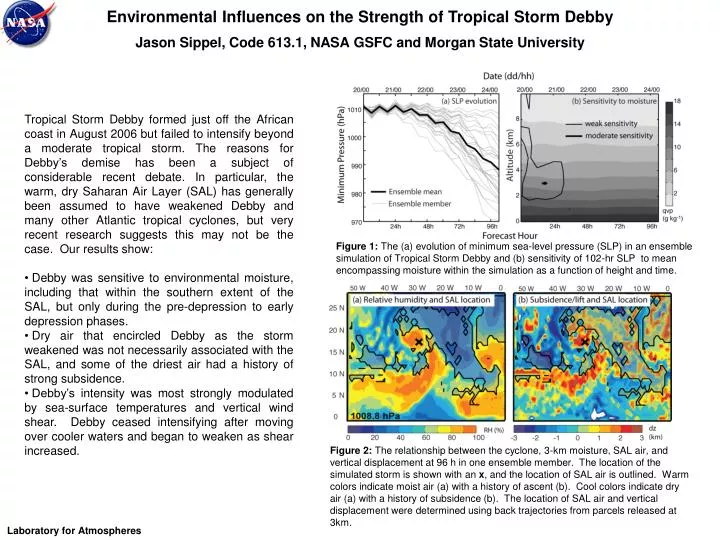
Environmental Influences on the Strength of Tropical Storm DebbyJason Sippel, Code 613.1, NASA GSFC and Morgan State University • Tropical Storm Debby formed just off the African coast in August 2006 but failed to intensify beyond a moderate tropical storm. The reasons for Debby’s demise has been a subject of considerable recent debate. In particular, the warm, dry Saharan Air Layer (SAL) has generally been assumed to have weakened Debby and many other Atlantic tropical cyclones, but very recent research suggests this may not be the case. Our results show: • Debby was sensitive to environmental moisture, including that within the southern extent of the SAL, but only during the pre-depression to early depression phases. • Dry air that encircled Debby as the storm weakened was not necessarily associated with the SAL, and some of the driest air had a history of strong subsidence. • Debby’s intensity was most strongly modulated by sea-surface temperatures and vertical wind shear. Debby ceased intensifying after moving over cooler waters and began to weaken as shear increased. Figure 1: The (a) evolution of minimum sea-level pressure (SLP) in an ensemble simulation of Tropical Storm Debby and (b) sensitivity of 102-hr SLP to mean encompassing moisture within the simulation as a function of height and time. Figure 2: The relationship between the cyclone, 3-km moisture, SAL air, and vertical displacement at 96 h in one ensemble member. The location of the simulated storm is shown with an x, and the location of SAL air is outlined. Warm colors indicate moist air (a) with a history of ascent (b). Cool colors indicate dry air (a) with a history of subsidence (b). The location of SAL air and vertical displacement were determined using back trajectories from parcels released at 3km. Laboratory for Atmospheres (a) EnKF radar (a) EnKF radar (b) EnKF sfc winds (b) EnKF sfc winds (d) Pure ens sfc winds (d) Pure ens sfc winds (c) Pure ens radar (c) Pure ens radar
Name: Jason Sippel, NASA/GSFC, Code 613.1 and Morgan State University E-mail: jason.sippel@nasa.gov Phone: 301-614-6285 References: Sippel, J. A., S. A. Braun, and C.-L. Shie, 2011: Environmental influences on the strength of Tropical Storm Debby (2006). Journal of Atmospheric Sciences, in press. Braun, S. A., J. A. Sippel, and D. Nolan, 2011: The impact of dry Saharan air on hurricane intensity in idealized simulations with no mean flow. Conditionally accepted to the Journal of Atmospheric Sciences. Data Sources: MODIS, TRMM, AIRS, Modern Era Retrospective-Analysis (MERRA), NCEP Final Analysis. Technical Description of Figures: Figure 1: A nested high-resolution (3 km) ensemble of simulations of Debby was created with the Advanced Research version of the Weather Research and Forecasting model (WRF-ARW v2.1) by perturbing the NCEP FNL analysis with a set of 30 random, large scale perturbations and integrating for 102 h. Figure 1a shows the evolution of minimum SLP for all members and the ensemble mean for the duration of the ensemble. Sensitivity of 102-h cyclone intensity to differing environmental conditions was examined by computing the semi-partial correlation between 102-h SLP and various parameters and variables every 6 h. Figure 1 b shows ensemble mean water vapor within several hundred km of the cyclone and the sensitivity of 102-h SLP to variability in mean water vapor in the ensemble members. The averaging area for water vapor was decreased from a radius of 500 to 200 km from the beginning to end of the simulation to crudely represent the changing scale of the system. Later during the simulation, the sensitivity decreased because the circulation associated with the vortex likely prevented warm and dry environmental air from entraining into the system and disrupting convection. Figure 2: The relationship between the cyclone, 3-km moisture, SAL air, and the vertical displacement of 3-km air at 96 h in one ensemble member. The location of the simulated storm is shown with an x, and the location of SAL air is outlined. Warm colors indicate moist air (a) with a history of ascent (b). Cool colors indicate dry air (a) with a history of subsidence (b). The location of SAL air and vertical displacement were determined using back trajectories from parcels released at 3km. The trajectories were calculated from 15-minute output on domain 1 (i.e., the 27-km grid) and processed with RIP version 4.3. Air was determined to be of SAL origin based upon its initial starting coordinates and relative humidity in the model. Areas of SAL air are superposed upon the relative humidity field in Fig. 2a to illustrate the relationship between SAL air and moisture. Meanwhile, the net vertical displacement between 3 km and the initial altitude is shown in Fig. 2b to show where 3-km air has a history of subsidence or ascent. Scientific significance: The role of the SAL in cyclone intensity change is an area of current active research. A number of studies over the past decade have concluded, based on largely circumstantial evidence, that the SAL strongly modulates the strength of individual tropical cyclones and cyclone activity in general over the Atlantic basin. However, very recent research has shown that warm, dry air formerly presumed to be of SAL origin was actually a result of subsidence and did not originate over the Sahara. In addition, other research has shown that it is difficult for environmental air to entrain into the circulation of a mature tropical cyclone. This research is important because it quantifies the exact role of the SAL in modulating the intensity of a particular tropical cyclone. It also compares the influence of the SAL to the influence of other environmental factors that are known to affect tropical cyclones. Relevance for future science and relationship to Decadal Survey: Investigating the relationship between the SAL and tropical cyclones is a central focus of the upcoming Hurricane and Severe Storm Sentinel (HS3) field campaign. Laboratory for Atmospheres
Aerosol Observations and Cloud Contamination: Detection of thin cirrus bias using MPLNET Ellsworth Welton (613.1), Jingfeng Huang (613.2, GESTAR), Brent Holben (614.4), Si-Chee Tsay (613.2) • Aerosol-cloud interactions affect aerosol physical properties (i.e., size) and in turn their influence on solar radiation and possibly cloud formation and rainfall. The optical thickness of aerosols (AOT) and clouds is derived from passive satellite and ground instruments and is used to determine their influence on climate. It is important to accurately measure both aerosol and cloud optical thickness and avoid cloud contamination in AOT measurements. Data collected from the NASA Micro Pulse Lidar Network (MPLNET) are being used to provide cirrus cloud detection/heights with co-incident AOT measurements from the NASA Aerosol Robotic Network (AERONET). • Two recent studies of observations from South East Asia demonstrate the difficulty in screening thin clouds during passive aerosol observations. • When cirrus was present, AOT results were biased high and the retrieved aerosol size distributions show a corresponding increase in large particles. • A new improved AERONET data release is being developed. MPLNET cloud heights will be used to verify the performance of the new cloud screening procedure. (a) (b) (c) Figure 1: (a) MPLNET Level 1 lidar signals collected from Phimai, Thailand, on March 21-25, 2006. Black stripes are periods when the lidar was covered at solar noon to prevent damage to the instrument. (b) PDFs of AERONET Level 2 aerosol optical thickness (AOT) for all observations in April 2006 with (red) and without (blue) cirrus, based on detection from MPLNET data. (c) Average AERONET Level 2 aerosol size distributions for all observations in April-May 2006 with (red) and without (blue) cirrus, based on detection from MPLNET data. Laboratory for Atmospheres
Name: Ellsworth J. Welton, NASA/GSFC, Code 613.1 E-mail: Ellsworth.J.Welton@nasa.gov Phone: 301-614-6279 References: Huang, J., N. C. Hsu, S. Tsay, M. Jeong, B. N. Holben, T. A. Berkoff, and E. J. Welton, 2011. Susceptibility of aerosol optical thickness retrievals to thin cirrus contamination during the BASE-ASIA campaign, Journal of Geophysical Research, 116, D08214, doi:10.1029/2010JD014910. Boon-Ning, C., J.R. Campbell, J.S. Reid, D.M. Giles, E.J. Welton, S.V. Santos, and S.C. Liew, 2011: Tropical Cirrus Cloud Contamination in Sun Photometer Data, Atmospheric Environment, accepted. We also credit the excellent work performed by the AERONET and MPLNET staff, and our network partners worldwide. Data Sources: NASA MPLNET and AERONET networks, MODIS. Technical Description of Figures: Figure 1: (a) MPLNET Level 1 lidar signals collected from Phimai, Thailand, on March 21-25, 2006. Black stripes are periods when the lidar was covered at solar noon to prevent damage to the instrument. Cirrus clouds are persistent in South East Asia, and this region was ideal for assessing cloud contamination issues. The MPLNET data here provide an example of data collected in the region. Wide spread cirrus are present over relatively thick and turbid aerosol layers (predominantly smoke here). (b) PDFs of AERONET Level 2 aerosol optical thickness (AOT) for all observations in April 2006 with (red) and without (blue) cirrus, based on detection from MPLNET data. (c) Average AERONET Level 2 aerosol size distributions for all observations in April-May 2006 with (red) and without (blue) cirrus, based on detection from MPLNET data. Plots (b) and (c) are from Huang et al (2011) and illustrate the thin cirrus bias in the current operational Level 2 AERONET AOT product from sites such as Phimai. The same analysis was applied to measurements constrained to 1000-1400 local time to minimize view angle differences between the lidar (nadir) and the sunphotometer (solar zenith angle) and the results still show a significant thin cirrus bias at a 95% confidence level (Kolmogorov-Smirnov (KS) statistical test). Scientific significance: Aerosols and clouds scatter and absorb sunlight, thereby influencing the Earth’s radiation balance. Aerosol-cloud interactions affect aerosol physical properties (i.e., size) and in turn their influence on solar radiation and possibly cloud formation and rainfall. Aerosol-cloud interactions are both very significant and also very uncertain (IPCC), the latter due to the inhomogeneous composition and distribution of aerosols and clouds, and their relatively short lifetimes. The optical thickness of aerosols (AOT) and clouds, a parameter proportional to the concentration, is derived from passive satellite and ground instruments and is used to determine their influence on climate. It is important to accurately measure both aerosol and cloud optical depths, and in particular to avoid cloud contamination in AOT measurements. Data collected from the NASA Micro Pulse Lidar Network (MPLNET) are being used to provide cirrus cloud detection/heights with co-incident AOT measurements from the NASA Aerosol Robotic Network (AERONET). Results from a recent study of observations from South East Asia demonstrate the difficulty in screening thin clouds during passive aerosol observations. A similar study for results from Singapore has been accepted for publication. MPLNET cloud heights will be used to verify the performance of the new AERONET cloud screening procedure. Relevance for future science and relationship to Decadal Survey: The results of the current efforts will contribute to the development of the new improved Version 3 AERONET data release. The information obtained on thin cirrus bias in passive AOT retrievals will inform current missions, such as MODIS on Aqua and Terra, as well as future aerosol missions such as PACE/ACE. Laboratory for Atmospheres
Low Clouds Aid Sea Ice Loss Dong L. Wu, Code 613.2, NASA GSFC, and Jae N. Lee, Caltech/JPL, Pasadena, CA 10-yr Trend in the BESS Region MISR Mean Cloud Cover (0-3km) 10-yr Trend of Cloud Cover (0-3km) Barents Sea East Siberian Sea Beaufort Sea • Figure 1 • The Beaufort and East Siberian Sea (BESS) shows a large increase in surface air temperature in the recent decade for months of Sep-Nov. Figure 2 Major Findings: • Terra/MISR data reveals a significant increase of low cloud cover in October during 2000-2010, the largest in the daylight Arctic months (March-October), and the result is consistent with CALIPSO lidar observations since 2006. • The regions with the largest October low cloud increase collocate with where most sea ice loss occurred in Sep. • MISR cloud observations support the theorized positive ice-temperature-cloud feedback, whereby more open water in the Arctic Ocean increases summer absorption of solar radiation, and subsequent evaporation, which leads to more low clouds in autumn. Trapping longwave radiation, these clouds effectively lengthen the melt season and reduce perennial ice pack formation, making sea ice more vulnerable to the next melt season. • Terra covers this important decade when an intensified warming occurred over the Arctic Ocean, and MISR observations provide valuable clues to the problem. • Causes of the warming remain unclear; but increased absorption of summer solar radiation and autumn low cloud formation have been suggested as a positive ice-temperature-cloud feedback in the Arctic. Laboratory for Atmospheres
Name: Dong L. Wu, NASA/GSFC Code 613.2E-mail: Dong.L.Wu@nasa.govPhone: 301-614-5784 References: Serreze, M. C., et al., The emergence of surface-based Arctic amplification. Cryosphere, 3, 11–19, 2009. Vavrus, S., et al., Changes in Arctic clouds during intervals of rapid sea ice loss. Clim Dyn, DOI 10.1007/s00382-010-0816-0, 2010. Data Sources: Terra/MISR and CALIPSO cloud fraction. Technical Description of Figures: Figure 1:Daily mean surface air temperature (SAT) from NCEP/NCAR reanalysis over the Beaufort-East Siberian Sea (110E-220E and 70N-80N), or BESS, for each decade since 1950.The Arctic warming reported in surface air temperature (SAT) occurs non-uniformly with season with the strongest increase in autumn [Serreze et al., 2009]. Over the Arctic Ocean, the BESS show the largest SAT increases in September-November, resembling the pattern of sea ice reduction in September. It was not until 2000-2009 that the autumn temperature increase becomes significantly above the envelope defined by previous decades. Figure 2: MISR low (0-3 km) cloud cover and trend for months of Sep and Oct of 2000-2010. (a) The mean low cloud cover is in color, overlaid by a thick black line for the border of 20% ice-free water in the month. The box indicates the BESS region of interest. (b) Trend maps of MISR low cloud cover in 2000-2010 with small (large) positive trend in Sep (Oct). (c) Trend of low cloud cover from BESS. Cyan lines are the CALIPSO lidar observations of low cloud fraction in the same region. Similar to lidar measurements, MISR cloud fraction is derived by discriminating features with a height above the surface. Different from other passive cloud detection techniques, MISR stereo is not limited by snowy/icy surfaces nor by radiometric calibration in the Arctic cloud case. Scientific significance: The observed increase of October low cloud cover over the Arctic Ocean support the hypothesis that low clouds have a positive feedback to sea ice loss by warming SAT during late summer and autumn, and thus reducing perennial ice pack formation. Relevance for future science and relationship to Decadal Survey: Monitoring and understanding the rapid climate changes in the polar region is one of NASA’s strategic goals in climate research. The multiangle imagers and lidar sensor on the NASA’s ACE mission will provide the similar cloud measurements presented in this study, but better coverage and sensitivity are anticipated. Laboratory for Atmospheres
Unusual Dynamical Conditions in the Arctic Stratosphere in March 2011Margaret M. Hurwitz, NASA GESTAR, Code 613.3, NASA GSFC Paul A. Newman, Code 613.3, NASA GSFC Chaim. I. Garfinkel, Johns Hopkins University In March 2011, the Arctic stratosphere was much colder than usual, leading to severe polar ozone depletion. March temperature in the Arctic stratosphere is highly correlated with tropospheric wave forcing in February (Newman et al., 2001). Meteorological reanalyses show that wave forcing in 2011 was much weaker than usual, consistent with the unusually cold conditions. Similarly weak wave forcing and March temperatures were observed in 1997. Dynamical conditions that are known to reduce wave activity and cool the Arctic stratosphere in mid-winter (specifically, La Niña and QBO-westerly; see Garfinkel et al., 2010) persisted throughout the 2010-2011 winter season. However, they do not explain the unusually cold Arctic stratosphere in March 2011. Sea surface temperatures (SSTs) in the North Pacific were warmer than usual in the late winter in both 1997 and 2011. The positive phase of this “subarctic SST mode” is associated with a cooler Arctic stratosphere in March. This result provides new evidence for interactions between the ocean and stratosphere and motivates a modeling study of the role of extra-tropical SSTs on Arctic variability. Figure 1: The top two panels show March temperature differences from climatology in the Northern Hemisphere troposphere and stratosphere. In 2011 and 1997, the Arctic stratosphere was approximately 10K colder than usual. The center panels show that typical La Niña and QBO-westerly conditions are not consistent with the cold conditions in March 2011. The lower panel shows that the positive phase of the subarctic SST mode may explain the unusually cold Arctic stratosphere in March 2011. Laboratory for Atmospheres
Name: Margaret M. Hurwitz, NASA GESTAR, Code 613.3, NASA GSFC E-mail: margaret.m.hurwitz@nasa.gov Phone: 301-614-6889 References: Garfinkel, C. I., D. L. Hartmann, and F. Sassi (2010). Tropospheric Precursors of Anomalous Northern Hemisphere Stratospheric Polar Vortices. Journal of Climate, 23, 3282-3299. Hurwitz, M. M., P. A. Newman, and C. I. Garfinkel (2011). The Arctic Vortex in March 2011: A Dynamical Perspective, submitted to Atmospheric Chemistry and Physics. Newman, P. A., E. R. Nash, and J. E. Rosenfield (2001). What controls the temperature of the Arctic stratosphere during the spring? Journal of Geophysical Research, 106, 19,999–20,010, doi:10.1029/2000JD000061. Data Sources: Atmospheric data were provided by various meteorological reanalyses, including NCEP-2, MERRA and CPC. Sea surface temperatures were taken from the HadISST1 dataset. Observational results were compared with GEOS Chemistry-Climate Model simulations. Technical Description of Figures: Figure 1: March temperature differences [K] in the NCEP-2 reanalysis. Top left: 2011 from the 1979-2011 climatological mean. Top right: 1997 from the climatological mean. Center left: Composite of La Niña events from the climatological mean. Center right: QBO-westerly as compared with QBO-easterly years. Lower panel: March temperature differences for years when subarctic SSTs in the 40-50°N, 160-200°E region are more (less) than one standard deviation greater (less than) the climatological mean. In the center and lower panels, black Xs denote differences significant at the 95% confidence level. Zero difference contours are shown in white. Scientific significance: The Arctic stratosphere is highly variable in winter, both on interseasonal and interannual timescales. Understanding and attributing this variability can improve the predictability of stratospheric ozone depletion and weather patterns at Northern Hemisphere mid- and high latitudes. While tropical sea surface temperature (SST) variability (i.e., El Niño and La Niña events) is known to contribute to stratospheric variability, this work is the first to show that extra-tropical SSTs also affect the Arctic stratosphere in late winter. SST anomalies in the North Pacific in January and February weaken planetary wave forcing in February, reducing temperatures in the Arctic stratosphere in March. Also, this work shows the need to separate mid-winter conditions from those in late winter (March). While La Niña events tend to cool the Arctic stratosphere in November through February, the sign of stratospheric temperature anomalies begins to reverse in March. Relevance for future science and relationship to Decadal Survey: This result provides new evidence for interactions between the ocean and stratosphere and motivates a modeling study of the role of extra-tropical SSTs on Arctic variability. A chemistry-climate model with a coupled ocean, currently in development at NASA GSFC, will provide the ideal tool for this study. Laboratory for Atmospheres