Bivariate Data
Bivariate Data. Pick up a formula sheet, Notes for Bivariate Data – Day 1, and a calculator.

Bivariate Data
E N D
Presentation Transcript
Bivariate Data Pick up a formula sheet, Notes for Bivariate Data – Day 1, and a calculator.
Archaeopteryx is an extinct beast having feathers like a bird but teeth and a long bony tail like a retile. Only six fossil specimens are known. Because these specimens differ greatly in size, some scientists think they are different species rather than individuals from the same species. If the specimens belong to the same species and differ in size because some are younger than others, there should be a positive linear relationship between the bones from all individuals. An outlier from this relationship would suggest a different species. Here are data on the lengths in centimeters of the femur (a leg bone) and the humerus (a bone in the upper arm) for the five specimens that preserve both bones. Load data into list 1 and list 2 and make a scatterplot.
72 humerus length in cm 41 64 38 femur length in cm A “cheater” way to put scale on a scatterplot is to trace two points and label each axis with those two values.
72 humerus length in cm 41 64 38 femur length in cm explanatory variable? femur length in cm response variable? humerus length in cm But does it really matter here? No. But often it does.
Find the correlation coefficient and explain what it means. correlation coefficient Did you get it?
If you did not get the correlation coefficient, you must turn your diagnostics on. Push 2nd then 0. Scroll down to diagnostics on. Push “enter” twice and little calculator guy will say “done”.
Find the correlation coefficient and explain what it means. correlation coefficient
r = .994 The correlation coefficient is ALWAYS between -1 and 1. It does not change when the units or scale is transformed. Let’s check out the formula sheet.
r = .994 What does it mean? The correlation coefficient describes the strength of the linear relationship. The closer it is to 1 or -1 the more the points line up. These points line up pretty well with a negative slope. The correlation coefficient would be close to -1. graph on the bottom of your notes
r = .994 What does it mean? The correlation coefficient describes the strength of the linear relationship. The closer it is to 1 or -1 the more the points line up. These points line up pretty well with a positive slope. The correlation coefficient would be close to 0.8 or 0.9.
r = .994 What does it mean? The correlation coefficient describes the strength of the linear relationship. The closer it is to 1 or -1 the more the points line up. These points don’t line up at all. The correlation coefficient would be nearly 0.
r = .994 What does it mean? The correlation coefficient describes the strength of the linear relationship. The closer it is to 1 or -1 the more the points line up. These points line up sort of well with a negative slope. The correlation coefficient might be – 0.6 or – 0.7.
r = .994 What does it mean? The correlation coefficient describes the strength of the linear relationship. The closer it is to 1 or -1 the more the points line up. These points don’t line up at all. The correlation coefficient would be fairly close to 0.
r = .994 Here’s what you write: This suggests a strong, positive,linear relationship between femur length and humerus length.
slope y-intercept coefficient of determination equation: ŷ = 1.197x – 3.660 This is hugely important! It means the predicted y.
equation: ŷ = 1.197x – 3.660 where x = femur length and y = humerus length slope = 1.197 ; For every 1 cm increase in femur length, the humerus length increases by 1.197 cm, on average. y-intercept ; When the femur length is 0 cm, the humerus length is about -3.660 cm. Of course, this is ridiculous and is an example of extrapolation.
y ŷ ŷ y Residuals A residual is the distance between the actual point and the predicted point. residual = y – ŷ since the point is above the line, the residual will be positive since the point is below the line, the residual will be negative
What is the residual for the point (38, 41)? residual = y – ŷ First find y. 41
What is the residual for the point (38, 41)? residual = 41 – ŷ Then find ŷ using the equation of the line. ŷ = 1.197x – 3.660 ŷ = 1.197(38) – 3.660 ŷ = 41.826 residual = 41 – 41.826 = – .826
What is the residual for the point (59, 70)? residual = 70 – 66.963 = 3.037
Residual Plot The residual plot is a scatterplot of all the residuals paired with their corresponding x values. residuals femur length
Residual Plot on the calculator Scroll down to L2 to get to the y-list.
Push 2nd – stat to get the list function. You should see resid. Enter resid. Remember: You need the equation of the line to find the residual. If you do not see “resid”, then you must first do the linear regression so the calculator knows which equation to use.
residuals femur length This is not the greatest residual plot. We would like the points to be randomly scattered about the line. Notice that the sum of the residuals will always be 0. Could push trace to get the actual points
residuals swine population Here’s a better residual plot from a different data set. It’s scattered randomly above and below the line.
What does a residual plot tell us? If points are randomly scattered above and below the line, then our linear equation is good. If there is a definite pattern, then another type of regression equation is more appropriate. Could be quadratic or exponential or logarithmic or any of the infinite mathematical possibilities.