Download
1 / 68
710 likes | 1.04k Views
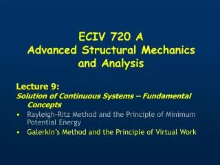
ECIV 720 A Advanced Structural Mechanics and Analysis. Lecture 15: Quadrilateral Isoparametric Elements (cont’d) Force Vectors Modeling Issues Higher Order Elements. Integration of Stiffness Matrix. B T (8x3). D (3x3). k e (8x8). B (3x8). Integration of Stiffness Matrix.

E N D
ECIV 720 A Advanced Structural Mechanics and Analysis Lecture 15: Quadrilateral Isoparametric Elements (cont’d) Force Vectors Modeling Issues Higher Order Elements
Integration of Stiffness Matrix BT(8x3) D(3x3) ke(8x8) B(3x8)
Integration of Stiffness Matrix Each term kij in ke is expressed as Linear Shape Functions is each Direction Gaussian Quadrature is accurate if We use 2 Points in each direction
Numerical Integration cannot produce exact results Accuracy of Integration is increased by using more integration points. Accuracy of computed FE solution DOES NOT necessarily increase by using more integration points. Choices in Numerical Integration
A quadrature rule of sufficient accuracy to exactly integrate all stiffness coefficients kij e.g. 2-point Gauss rule exact for polynomials up to 2nd order FULL Integration
Use of an integration rule of less than full order Reduced Integration, Underintegration Advantages • Reduced Computation Times • May improve accuracy of FE results • Stabilization • Disadvantages • Spurious Modes • (No resistance to nodal loads that tend to activate the mode)
Spurious Modes 8 degrees of freedom 8 modes Consider the 4-node plane stress element 1 t=1 E=1 v=0.3 1 Solve Eigenproblem
Spurious Modes Rigid Body Mode Rigid Body Mode
Spurious Modes Rigid Body Mode
Spurious Modes Flexural Mode Flexural Mode
Spurious Modes Shear Mode
Spurious Modes Uniform Extension Mode (breathing) Stretching Mode
Element Body Forces Total Potential Galerkin
Body Forces Integral of the form
Body Forces In both approaches Linear Shape Functions Use same quadrature as stiffness maitrx
Element Traction Total Potential Galerkin
Element Traction v Ty u Tx Similarly to triangles, traction is applied along sides of element 3 h 4 4 x 2 1
Traction Traction components along 2-3 For constant traction along side 2-3
Stresses h x More Accurate at Integration points Stresses are calculated at any x,h
Modeling Issues: Nodal Forces In view of… A node should be placed at the location of nodal forces Or virtual potential energy
Modeling Issues: Element Shape Square : Optimum Shape Not always possible to use Rectangles: Rule of Thumb Ratio of sides <2 Angular Distortion Internal Angle < 180o Larger ratios may be used with caution
Modeling Issues: Degenerate Quadrilaterals x 4 4 3 x x x x x x x 1 1 2 2 Integration Bias Coincident Corner Nodes 3 Less accurate
Modeling Issues: Degenerate Quadrilaterals Integration Bias 3 4 x 4 3 x x x x x 1 2 x x 1 2 Three nodes collinear Less accurate
Modeling Issues: Degenerate Quadrilaterals 2 nodes Use only as necessary to improve representation of geometry Do not use in place of triangular elements
A NoNo Situation h x Parent y (7,9) 3 (6,4) 4 2 1 J singular (3,2) (9,2) x All interior angles < 180
Another NoNo Situation x, y not uniquely defined h x
FEM at a glance It should be clear by now that the cornerstone in FEM procedures is the interpolation of the displacement field from discrete values Where m is the number of nodes that define the interpolation and the finite element and N is a set of Shape Functions
FEM at a glance 1 3 2 x x x1=-1 x1=-1 x2=1 x2=1 m=3 m=2
FEM at a glance 3 q6 v u q5 1 2 x 1 h 4 q4 q2 h q3 q1 2 x 3 m=3 m=4
FEM at a glance In order to derive the shape functions it was assumed that the displacement field is a polynomial of any degree, for all cases considered 1-D 2-D Coefficients ai represent generalized coordinates
FEM at a glance 1 3 2 x x1=-1 x2=1 For the assumed displacement field to be admissible we must enforce as many boundary conditions as the number of polynomial coefficients e.g.
FEM at a glance This yields a system of as many equations as the number of generalized displacements that can be solved for ai
FEM at a glance Substituting ai in the assumed displacement field and rearranging terms…
FEM at a glance 1 3 2 x x1=-1 x2=1 u(-1)=a0 -a1 +a2 =u1 … u(1)=a0 +a1 +a2 =u2 u(0)=a0 =u3 u(x)=a0+a1 x +a2 x2
Let’s go through the exercise 1 2 x1 x2 Assume an incomplete form of quadratic variation
Incomplete form of quadratic variation 1 2 x1 x2 We must satisfy
Incomplete form of quadratic variation And thus,
Incomplete form of quadratic variation And substituting in
Incomplete form of quadratic variation Which can be cast in matrix form as
Isoparametric Formulation 1 2 x1 x2 The shape functions derived for the interpolation of the displacement field are used to interpolate geometry
Intrinsic Coordinate Systems 4 (-1,1) 3 (1,1) h x 1 (-1,-1) 2 (1,-1) Intrinsic coordinate systems are introduced to eliminate dependency of Shape functions from geometry The price? Jacobian of transformation Great Advantage for the money!
Field Variables in Discrete Form Geometry Displacement Stress Tensor Strain Tensor s= DB un e= B un
FEM at a glance Element Strain Energy Work Potential of Body Force Work Potential of Surface Traction etc
Higher Order Elements Complete Polynomial 4 Boundary Conditions for admissible displacements Quadrilateral Elements Recall the 4-node 4 generalized displacements ai
Higher Order Elements Quadrilateral Elements Assume Complete Quadratic Polynomial 9 generalized displacements ai 9 BC for admissible displacements
9-node quadrilateral BT18x3 D3x3 B3x18 ke 18x18 9-nodes x 2dof/node = 18 dof
9-node element Shape Functions 4 3 Corner Nodes h 7 6 9 8 Mid-Side Nodes x 5 1 2 Middle Node Following the standard procedure the shape functions are derived as
9-node element – Shape Functions 1 3 2 x x1=-1 x2=1 Can also be derived from the 3-node axial element
Construction of Lagrange Shape Functions 1 (-1,-1) h (1,h) x (1,1)