Download
1 / 68
680 likes | 762 Views
Learn about hypothesis formulation in epidemiology, biostatistics, and analytical epidemiology. Explore the guidelines and primary steps for hypothesis testing in health sciences. Understand the role of null and alternative hypotheses in scientific research.

E N D
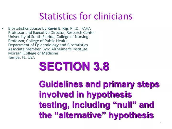
Statistics for clinicians • Biostatistics course by Kevin E. Kip, Ph.D., FAHAProfessor and Executive Director, Research CenterUniversity of South Florida, College of NursingProfessor, College of Public HealthDepartment of Epidemiology and BiostatisticsAssociate Member, Byrd Alzheimer’s InstituteMorsani College of MedicineTampa, FL, USA SECTION 3.8 Guidelines and primary steps involved in hypothesis testing, including “null” and the “alternative” hypothesis
Hypothesis Formulation Scientific Method (not unique to health sciences) --- Formulate a hypothesis --- Test the hypothesis
Basic Strategy of Analytical Epidemiology • 1. Identify variables you are interested in: • • Exposure • • Outcome • Formulate a hypothesis • 3. Compare the experience of two groups of subjects with respect to the exposure and outcome
Basic Strategy of Analytical Epidemiology • Hypothesis Testing • Two competing hypotheses • --- “Null” hypothesis (no association) – typically, but not always assumed • --- “Alternative” hypothesis (postulates there is an association) • Hypothesis testing is based on probability theory and the Central Limit Theorem
Hypothesis Formulation The “Biostatistician’s” way H0: “Null” hypothesis (assumed) H1: “Alternative” hypothesis The “Epidemiologist’s” way Direct risk estimate (e.g. best estimate of risk of disease associated with the exposure).
Hypothesis Formulation Biostatistician: H0: There is no associationbetween the exposure and disease of interest H1: There is an association between the exposure and disease of interest (beyond what might be expected from random error alone)
Hypothesis Formulation Epidemiologist: What is the best estimate of the risk of disease in those who are exposed compared to those who are unexposed (i.e. exposed are at XX times higher risk of disease). This moves away from the simple dichotomy of yes or no for an exposure/disease association – to the estimated magnitude of effect irrespective of whether it differs from the null hypothesis.
Hypothesis Formulation “Association” Statistical dependence between two variables: • Exposure (risk factor, protective factor, predictor variable, treatment) • Outcome (disease, event)
Hypothesis Formulation “Association” The degree to which the rate of disease in persons with a specific exposure is either higher or lower than the rate of disease among those without that exposure.
Hypothesis Formulation Ways to Express Hypotheses: 1. Suggest possible events… The incidence of tuberculosis will increase in the next decade.
Hypothesis Formulation Ways to Express Hypotheses: 2. Suggest relationship between specific exposure and health-related event… A high cholesterol intake is associated with the development (risk) of coronary heart disease.
Hypothesis Formulation Ways to Express Hypotheses: 3. Suggest cause-effect relationship…. Cigarette smoking is a cause of lung cancer
Hypothesis Formulation Ways to Express Hypotheses: 4. “One-sided” vs. “Two-sided” One-sided example: Helicobacter pylori infection is associated with increasedrisk of stomach ulcer Two-sided example: Weight-lifting is associated with risk of lower back injury
Hypothesis Formulation • Guidelines for Developing Hypotheses: • State the exposure to be measured as • specifically as possible. • State the health outcome as • specifically as possible. • Strive to explain the smallest amount • of ignorance
Hypothesis Formulation Example Hypotheses: POOR Eating junk food is associated with the development of cancer. GOOD The human papilloma virus (HPV) subtype 16 is associated with the development of cervical cancer.
SECTION 3.9 Parameters used in hypothesis testing
Level of significance: A fixed value of the probability of rejecting the null hypothesis (in favor of the alternative) when the null hypothesis is actually true (i.e. type I or alpha (α) error rate) Common levels of significance: 0.10, 0.05, 0.01, 0.001 α = 0.05: The probability of incorrectly rejecting the null hypothesis in favor of the alternative is 5% when the null hypothesis is true. P-value: A calculated probability of obtaining a test statistic at least as extreme as the one that was actually observed, assuming that the null hypothesis is true. A low p-value means that it is unlikely that the null hypothesis is actually true, and the alternative hypothesis should be considered (e.g. “reject” the null hypothesis).
Relative Relative Risk Risk 0.0 0.25 0.50 0.75 2.0 4.0 5.0 3.0 1.0 H H H 1 1 0 Null Alternative Alternative hypothesis hypothesis hypothesis PA < PB < PC > PD > PE A B C D E
Refer to the figure below. • Assume that 3 studies (A, B, and C) are conducted all with the same sample size. Which of the following is most likely true? • Study B will have a lower p-value than Study C • Study C will have the lowest p-value • None of the studies will be statistically significant • None of the above
Refer to the figure below. • Assume that 3 studies (A, B, and C) are conducted all with the same sample size. Which of the following is most likely true? • Study B will have a lower p-value than Study C • Study C will have the lowest p-value • None of the studies will be statistically significant • None of the above
Interpreting Results The p-value is NOT the index of causality It is an arbitrary quantity with no direct relationship to biology
SECTION 3.10 Type I and Type II error and factors that impact statistical power
Interpreting Results Four possible outcomes of any epidemiologic study:
Interpreting Results When evaluating the incidence of disease between the exposed and non-exposed groups, we need guidelines to help determine whether there is a true difference between the two groups, or perhaps just random variation from the study sample.
Interpreting Results “Conventional” Guidelines: • Set the fixed alpha level (Type I error) to 0.05 This means, if the null hypothesis is true, the probability of incorrectly rejecting it is 5% of less. The “p-value” is a measure of the compatibility of the data and the null hypothesis.
Interpreting Results Example: IE+ = 15 / (15 + 85) = 0.15 IE- = 10 / (10 + 90) = 0.10 RR = IE+/IE- = 1.5, p = 0.30 Although it appears that the incidence of disease may be higher in the exposed than in the non-exposed (RR=1.5), the p-value of 0.30 exceeds the fixed alpha level of 0.05. This means that the observed data are relatively compatible with the null hypothesis. Thus, we do not reject H0 in favor of H1 (alternative hypothesis).
Interpreting Results Conventional Guidelines: • Set the fixed beta level (Type II error) to 0.20 This means, if the null hypothesis is false, the probability of not rejecting it is 20% of less. The “power” of a study is (1 – beta). This means having 80% probability to reject H0 when H1 is true.
Interpreting Results Example: With the above sample size of 400, and if the alternative hypothesis is true, we need to expect a RR of about 2.1 (power = 82%) or higher to be able to reject the null hypothesis in favor of the alternative hypothesis.
Interpreting Results Factors that affect the power of a study: • 1. The fixed alpha level (the lower the level, the • the lower the power). • 2. The total and within group sample sizes (thesmaller the sample size, the lower the power -- • unbalanced groups have lower power than • balanced groups). • The anticipated effect size (the higher the • expected/observed effect size, the higher the power).
Interpreting Results Trade-offs between fixed alpha and beta levels: Reducing the fixed alpha level (e.g. to < 0.01) is considered “conservative.” This reduces the likelihood of a type I error (erroneously rejecting the null hypothesis), but at the expense of increasing the probability of a type II error if the alternative hypothesis is true.
Interpreting Results Trade-offs between fixed alpha and beta levels: Increasing the fixed alpha level (e.g. to < 0.10) reduces the probability of a type II error (failing to reject H0 when H1 is true), but at the expense of increasing the probability of a type I error if the null hypothesis is true.
Interpreting Results * Power with given sample size and risk ratio ( = 0.05) ** Risk ratio needed for 80% power with given sample size
SECTION 3.11 Calculate and interpret sample hypotheses – one sample continuous outcome
General Steps for Hypothesis Testing: • Set up the hypothesis and determine the level of statistical significance (including 1 versus 2-sided hypothesis). • Select the appropriate test statistic • Set up the decision rule • Compute the test statistic • Conclusion (interpretation)
1. Hypothesis Testing – One Sample Continuous Outcome • Compare a “historical control” mean (µ0) from a population to a “sample” mean. • Example: Average annual health care expenses per person in the year 2005 (n=100, X = $3,190, s = $890) are lower than “historical” control costs in the year 2002 ($3,302) • 1) Set up the hypothesis and determine the level of statistical significance (including 1 versus 2-sided hypothesis). • H0: µ = $3,302 • H1: µ < $3,302 (one-sided hypothesis, lower-tailed test) • α = 0.05
1. Hypothesis Testing – One Sample Continuous Outcome Example: Average annual health care expenses per person in the year 2005 (n=100, X = $3,190, s = $890) are lower than “historical” control costs in the year 2002 ($3,302) 2) Select the appropriate test statistic. If (n < 30), then use t If (n > 30), then use z
1. Hypothesis Testing – One Sample Continuous Outcome Example: Average annual health care expenses per person in the year 2005 (n=100, X = $3,190, s = $890) are lower than “historical” control costs in the year 2002 ($3,302) 3) Set up the decision rule (look up z value – Table 1c). Reject H0 if z< -1.645 4) Compute the test statistic: 3190 - 3302 z = --------------- = -1.26 890 / 100 5) Conclusion: -1.26 > -1.645 (critical value): Do not reject H0 Note: we cannot confirm the null hypothesis because perhaps the sample size was too small for a conclusive result (i.e. low power)
1. One Sample Continuous Outcome (Practice) • Compare historical “control” mean (µ0) from a population to a “sample” mean. • Example: Total cholesterol levels in the Framingham Heart Study in the year 2002 (n=3,310, X = 200.3, s = 36.8) are different than the national average in 2002 (203.0) • 1) Set up the hypothesis and determine the level of statistical significance (including 1 versus 2-sided hypothesis). • H0: µ = ______ • H1: µ ______ (???-sided hypothesis, ???-tailed test) • α = 0.05
1. One Sample Continuous Outcome (Practice) • Compare historical “control” mean (µ0) from a population to a “sample” mean. • Example: Total cholesterol levels in the Framingham Heart Study in the year 2002 (n=3,310, X = 200.3, s = 36.8) are different than the national average in 2002 (203.0) • 1) Set up the hypothesis and determine the level of statistical significance (including 1 versus 2-sided hypothesis). • H0: µ = 203 • H1: µ = 203 (2-sided hypothesis, 2-tailed test) • α = 0.05
1. One Sample Continuous Outcome (Practice) Example: Total cholesterol levels in the Framingham Heart Study in the year 2002 (n=3,310, X = 200.3, s = 36.8) are different than the national average in 2002 (203.0) 2) Select the appropriate test statistic. If (n < 30), then use t If (n > 30), then use z 3) Set up the decision rule (look up ??? value – Table 1c). Reject H0 if ______________________________ 4) Compute the test statistic: 5) Conclusion:
1. One Sample Continuous Outcome (Practice) Example: Total cholesterol levels in the Framingham Heart Study in the year 2002 (n=3,310, X = 200.3, s = 36.8) are different than the national average in 2002 (203.0) 2) Select the appropriate test statistic. If (n < 30), then use t If (n > 30), then use z 3) Set up the decision rule (look up z value – Table 1c). Reject H0 if z< -1.96 or if z> 1.96 4) Compute the test statistic: 200.3 - 203 z = --------------- = -4.22 36.8 / 3310 5) Conclusion: Reject H0 because -4.22 < -1.96 What about statistical versus clinical significance?
SECTION 3.12 Calculate and interpret sample hypotheses – one sample dichotomous outcome
2. Hypothesis Testing – One Sample Dichotomous Outcome • Compare a “historical control” proportion (p) from a population to a “sample” proportion. • Note: The example below assumes a “large” sample defined as: • np0 > 5 andn(1-p0) > 5 • If not, then “exact” methods must be used. • Example: The prevalence of smoking in the 2002 Framingham Heart Study (n=3,536, p = 482/3,536 = 0.1363) is lower than a national (“historical”) report in the year 2002 (p=0.211) • 1) Set up the hypothesis and determine the level of statistical significance (including 1 versus 2-sided hypothesis). • H0: p = 0.211 • H1: p < 0.211 (one-sided hypothesis, lower-tailed test) • α = 0.05
2. Hypothesis Testing – One Sample Dichotomous Outcome Example: The prevalence of smoking in the 2002 Framingham Heart Study (n=3,536, p = 482/3,536 = 0.1363) is lower than a national (“historical”) report in the year 2002 (p=0.211) 2) Select the appropriate test statistic. p – p0 z = ---------------- p0(1-p0) / n
2. Hypothesis Testing – One Sample Dichotomous Outcome Example: The prevalence of smoking in the 2002 Framingham Heart Study (n=3,536, p = 482/3,536 = 0.1363) is lower than a national (“historical”) report in the year 2002 (p=0.211) 3) Set up the decision rule (look up z value – Table 1c). Reject H0 if z< -1.645 4) Compute the test statistic: p – p0 z = ---------------- p0(1-p0) / n 0.136 – 0.211 z = ---------------------------- = -10.93 0.211(1-0.211) / 3,536 5) Conclusion: -10.93 < -1.645 (critical value): Reject H0
2. One Sample Dichotomous Outcome (Practice) • Compare historical “control” proportion (p) from a population to a “sample” mean. • Example: The prevalence of diabetes in a Tampa-based study of adults in 2002 (n=1,240, p = 108/1,240 = 0.0871) is different than a national (“historical”) report in the year 2002 (p=0.1082) • 1) Set up the hypothesis and determine the level of statistical significance (including 1 versus 2-sided hypothesis). • H0: p = ______ • H1: p ______ (???-sided hypothesis, ???-tailed test) • α = 0.05
2. One Sample Dichotomous Outcome (Practice) • Compare historical “control” proportion (p) from a population to a “sample” mean. • Example: The prevalence of diabetes in a Tampa-based study of adults in 2002 (n=1,240, p = 108/1,240 = 0.0871) is different than a national (“historical”) report in the year 2002 (p=0.1082) • 1) Set up the hypothesis and determine the level of statistical significance (including 1 versus 2-sided hypothesis). • H0: p=0.1082 • H1: p =0.1082 (2-sided hypothesis, 2-tailed test) • α = 0.05
2. One Sample Dichotomous Outcome (Practice) Example: The prevalence of diabetes in a Tampa-based study of adults in 2002 (n=1,240, p = 108/1,240 = 0.0871) is different than a national (“historical”) report in the year 2002 (p=0.1082) 2) Select the appropriate test statistic (assume z – large sample) 3) Set up the decision rule (look up z value – Table 1c). Reject H0 if _______________________ 4) Compute the test statistic: p – p0 z = ---------------- p0(1-p0) / n 5) Conclusion:
2. One Sample Dichotomous Outcome (Practice) Example: The prevalence of diabetes in a Tampa-based study of adults in 2002 (n=1,240, p = 108/1,240 = 0.0871) is different than a national (“historical”) report in the year 2002 (p=0.1082) 2) Select the appropriate test statistic (assume z – large sample) 3) Set up the decision rule (look up z value – Table 1c). Reject H0 if z< -1.96 or if z> 1.96 4) Compute the test statistic: p – p0 z = ---------------- p0(1-p0) / n 0.0871 – 0.1082 z = ---------------------------- = -2.39 0.1082(1-0.1082)/1,240 5) Conclusion: -2.39 < -1.96 (critical value): Reject H0
SECTION 3.13 Calculate and interpret sample hypotheses – one sample categorical/ordinal outcome