A semi-analytical ocean color inherent optical property model: approach and application.

1. A semi-analytical ocean color inherent optical property model: approach and application. Tim Smyth, Gerald Moore, Takafumi Hirata and Jim Aiken Plymouth Marine Laboratory, UK

2. Model description Implementation Validation Sensitivity study - summary Application to satellite data Further work Overview

3. Morel (1980): “ … the inverse system can be theoretically solved using simultaneous equations, if a spectral law is assumed for backscattering.” Not implemented (or implementable!) for either in situ or satellite data Sugihara & Kishino (1988) and Roesler & Perry (1995): implemented schemes for in-water reflectance data Not scaled up to satellite data (problems with Q) We have developed a scheme using simultaneous equations: solved using empirically derived spectral slopes in combination with radiative transfer modelling. Interface terms (Fresnel and f/Q): angular and IOP dependency Total absorption: aph(λ), ad(λ), ay(λ) 1) Model description • Two unknowns of bbp(λ) and a(λ): therefore require two equations … achieve this using two neighbouring wavelengths (i, j) and empirically derived spectral slopes.

4. Simultaneous equations 1) Model description Spectral slope in total absorption Spectral slope in total backscatter • solve equations simultaneously for a(j) and bbp(j) – nasty maths! • then can solve for a(i) and bbp(i) using spectral slopes. • need to work out which wavelength pairing to use for spectral slopes – based on empirical data.

5. 1) Model description N=216 • Spectral slopes from COLORS dataset (predominantly coastal stations) • εa(490,510) converged to narrow range of values with low σ • εa(490,510) = 1.268; εbb(490,510) = 1.0202 • Is this because only 20 nm difference between bands? • observationally: chlorophyll-a has greatest effect between 400 – 470 nm; minor effect between 490 and 510 nm.

6. 1) Model description • Once have a(490,510) and bbp(490,510), then use assumed shape of backscatter to extrapolate to other wavelengths: • can then work out the entire spectrum of a(λ) • bio-geochemical parameters of ady(λ) and aph(λ) can be determined using spectral slope method • εdy(412,443) and εph(412,443) selected as they are distinct with low variance. Used in combination with standard CDOM exponential function to extrapolate to other wavelengths.

7. 2) Implementation

8. Validation using NOMAD in situ dataset: Points selected on basis that each entry contained ρw(SeaWiFS); a(λ); aph(λ) and ady(λ); 439 data points met this criterion; 88 data points for bbp(λ). Comparison with Lee et al. (2002) model 3) Validation

9. Signal to noise ratio? Raman scattering? 3) Validation: Total absorption (PML model), a(λ) R2: 0.835 RMS: 0.192 R2: 0.851 RMS: 0.161 R2: 0.840 RMS: 0.202 N=418 Good retrievals over 2 orders of magnitude R2: 0.819 RMS: 0.118 R2: 0.637 RMS: 0.148 R2:0.061 RMS: 0.362

10. Limitation at higher absorption 3) Validation: Total absorption (Lee model), a(λ) R2: 0.549 RMS: 0.362 R2: 0.464 RMS: 0.376 R2: 0.206 RMS: 0.415 N=439 R2: 0.006 RMS: 0.435 R2: 0.509 RMS: 0.475 R2: 0.556 RMS: 0.308

11. Increasing bias with increasing λ: problem with assumed spectral shape? 3) Validation: Total backscatter, bb(λ) R2: 0.395 RMS: 0.148 R2: 0.387 RMS: 0.192 R2: 0.400 RMS: 0.148 N=88 R2: 0.375 RMS: 0.270 R2: 0.354 RMS: 0.390 R2: 0.383 RMS: 0.217

12. 3) Validation: CDOM absorption, ady(λ) R2: 0.532 RMS: 0.500 R2: 0.568 RMS: 0.507 R2: 0.477 RMS: 0.516 R2: 0.453 RMS: 0.519 R2: 0.406 RMS: 0.538 R2: 0.313 RMS: 0.595 Noisy at low ady(λ): possible measurement error?

13. 3) Validation: phytoplankton absorption, aph(λ) R2: 0.744 RMS: 0.263 R2: 0.666 RMS: 0.298 R2: 0.759 RMS: 0.230 R2: 0.394 RMS: 0.857 R2: 0.677 RMS: 0.358 R2: 0.099 RMS: 0.178 Problems with retrievals at 555 and 670

14. a(λ) and bb(λ): Model most sensitive to εa(490,510) NOMAD 1.317 cf. COLORS 1.268 Relatively insensitive to εbb(490,510) NOMAD 1.040 cf. COLORS 1.0202 ady(λ) and aph(λ) Most sensitive to εph(412,443) NOMAD 1.065 cf. COLORS 0.954 Relatively insensitive to εdy(412,443) and S NOMAD 1.638 cf. COLORS 1.579 4) Sensitivity study - summary

15. Implemented on HRPT and GAC SeaWiFS imagery using an Intel Xeon 1.8 GHz processor: 15 mins proc HRPT 1.5 mins process on GAC entire orbit 5) Application to satellite data

16. CDOM bloom? Sediment Coccolithophores Phytoplankton – fine eddy structure Clear blue ocean 18 May 1998 13.14 GMT “True color” composite - qualitative

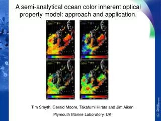
17. a(443) ady(443) • a(443): high values (0.2 – 0.5 m-1) in coastal seas; ca. 0.3 m-1 in bloom. • ady(443): coastal seas dominated by CDOM; • aph(443): phytoplankton bloom off W. Ireland; • bbp(555): Emiliana huxleyi bloom in Western Approaches (in situ confirmed this) • IOP model allows us to quantify these features. aph(443) bbp(555)

18. 10 Oct 2002 10.26 GMT Namibia South Africa a(443) aph(443) ady(443) • BENCAL experiment (October 2002) • upwelling combination of ady and aph; offshore bloom dominated by aph

19. 490:510 pairing used for SeaWiFS / MERIS Develop 488:532 spectral slopes for use with MODIS 412:443 pair for ady and aph subject to ρw(412) problems (atmospheric correction); could use 443:490 pairing instead IOP models can form building block for many applications: Determination of phytoplankton functional types; Data assimilation into process oriented models: address rate equations, cf. chlorophyll which is a model derived variable; Primary production modelling without recourse to chlorophyll 5) Further work