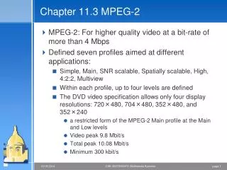
Chapter 11.3 MPEG-2

1. Chapter 11.3 MPEG-2 • MPEG-2: For higher quality video at a bit-rate of more than 4 Mbps • Defined seven profiles aimed at different applications: • Simple, Main, SNR scalable, Spatially scalable, High, 4:2:2, Multiview • Within each profile, up to four levels are defined • The DVD video specification allows only four display resolutions: 720×480, 704×480, 352×480, and 352×240 • a restricted form of the MPEG-2 Main profile at the Main and Low levels • Video peak 9.8 Mbit/s • Total peak 10.08 Mbit/s • Minimum 300 kbit/s

3. Supporting Interlaced Video • MPEG-2 must support interlaced video as well since this is one of the options for digital broadcast TV and HDTV • In interlaced video each frame consists of two fields, referred to as the top-field and the bottom-field • In a Frame-picture, all scanlines from both fields are interleaved to form a single frame, then divided into 16×16 macroblocks and coded using MC • If each field is treated as a separate picture, then it is called Field-picture • MPEG 2 defines Frame Prediction and Field Prediction as well as five prediction modes

4. Fig. 11.6: Field pictures and Field-prediction for Field-pictures in MPEG-2. • (a) Frame−picture vs. Field−pictures, (b) Field Prediction for Field−pictures

5. Zigzag and Alternate Scans of DCT Coefficients for Progressive and Interlaced Videos in MPEG-2.

6. MPEG-2 layered coding • The MPEG-2 scalable coding: A base layer and one or more enhancement layers can be defined • The base layer can be independently encoded, transmitted and decoded to obtain basic video quality • The encoding and decoding of the enhancement layer is dependent on the base layer or the previous enhancement layer • Scalable coding is especially useful for MPEG-2 video transmitted over networks with following characteristics: • – Networks with very different bit-rates • – Networks with variable bit rate (VBR) channels • – Networks with noisy connections

7. MPEG-2 Scalabilities • MPEG-2 supports the following scalabilities: • SNR Scalability—enhancement layer provides higher SNR • Spatial Scalability — enhancement layer provides higher spatial resolution • Temporal Scalability—enhancement layer facilitates higher frame rate • Hybrid Scalability — combination of any two of the above three scalabilities • Data Partitioning — quantized DCT coefficients are split into partitions

8. Major Differences from MPEG-1 • Better resilience to bit-errors: In addition to Program Stream, a Transport Stream is added to MPEG-2 bit streams • Support of 4:2:2 and 4:4:4 chroma subsampling • More restricted slice structure: MPEG-2 slices must start and end in the same macro block row. In other words, the left edge of a picture always starts a new slice and the longest slice in MPEG-2 can have only one row of macro blocks • More flexible video formats: It supports various picture resolutions as defined by DVD, ATV and HDTV

9. Other Major Differences from MPEG-1 (Cont’d) • Nonlinear quantization — two types of scales: • For the first type, scale is the same as in MPEG-1 in which it is an integer in the range of [1, 31] and scalei= i • For the second type, a nonlinear relationship exists, i.e., scalei≠i. The ith scale value can be looked up from Table

10. Chapter 12: MPEG – 4 and beyond • 12.5: H.264 = MPEG-4 Part 10, or MPEG-4 AVC • H.264 offers up to 30-50% better compression than MPEG-2, and up to 30% over H.263+ and MPEG-4 advanced simple profile • Core Features • VLC-Based Entropy Decoding: Two entropy methods are used in the variable-length entropy decoder: Unified-VLC (UVLC) and Context Adaptive VLC (CAVLC) • Motion Compensation (P-Prediction): Uses a tree-structured motion segmentation down to 4×4 block size (16×16, 16×8, 8×16, 8×8, 8×4, 4×8, 4×4). This allows much more accurate motion compensation of moving objects. Furthermore, motion vectors can be up to half-pixel or quarter-pixel accuracy • Intra-Prediction (I-Prediction): H.264 exploits much more spatial prediction than in H.263+

11. P and I prediction schemes are accurate. Hence, little spatial correlation let. H.264 therefore uses a simple integer-precision 4 × 4 DCT, and a quantization scheme with nonlinear step-sizes • In-Loop Deblocking Filters

12. Baseline Profile Features • The Baseline profile of H.264 is intended for real-time conversational applications, such as videoconferencing • Arbitrary slice order (ASO): decoding order need not be monotonically increasing – allowing for decoding out of order packets • Flexible macroblock order (FMO) – can be decoded in any order – lost macroblocks scattered throughout the picture • Redundant slices to improve resilience

13. Main Profile Features • Represents non-low-delay applications such as broadcasting and stored-medium • B slices: B frames can be used as reference frames. They can be in any temporal direction (forward-forward, forward-backward, backward-backward) • More flexible - 16 reference frames (or 32 reference fields) • Context Adaptive Binary Arithmetic Coding (CABAC) • Weighted Prediction • Not all decoders support all the features • http://en.wikipedia.org/wiki/H.264/MPEG-4_AVC

14. MPEG-4 • MPEG-4 adopts a object-based coding: • Offering higher compression ratio, also beneficial for digital video composition, manipulation, indexing, and retrieval • The bit-rate for MPEG-4 video now covers a large range between 5 kbps to 10 Mbps • More interactive than MPEG-1 and MPEG-2

15. Composition and manipulation of object

16. Overview of MPEG-4 • Video-object Sequence (VS)—delivers the complete MPEG-4 visual scene, which may contain 2-D or 3-D natural or synthetic objects • Video Object (VO) — a object in the scene, which can be of arbitrary shape corresponding to an object or background of the scene • Video Object Layer (VOL) — facilitates a way to support (multi-layered) scalable coding. A VO can have multiple VOLs under scalable coding, or have a single VOL under non-scalable coding • Group of Video Object Planes (GOV) — groups Video Object Planes together (optional level) • Video Object Plane (VOP) — a snapshot of a VO at a particular moment

17. Comparison between Block-based Coding and Object-based Coding

18. Object oriented • VOP – I-VOP, B-VOP, P-VOP • Objects can be arbitrary shape – need to encode the shape and the texture (object) • Need to treat MB inside object different than boundary blocks (padding, different DCT etc)

19. Sprite Coding • A sprite is a graphic image that can freely move around within a larger graphic image or a set of images • To separate the foreground object from the background, we introduce the notion of a sprite panorama: a still image that describes the static background over a sequence of video frames • The large sprite panoramic image can be encoded and sent to the decoder only once at the beginning of the video sequence • When the decoder receives separately coded foreground objects and parameters describing the camera movements thus far, it can reconstruct the scene in an efficient manner

21. Global Motion Compensation (GMC) • “Global” – overall change due to camera motions (pan, tilt, rotation and zoom) • Without GMC this will cause a large number of significant motion vectors • There are four major components within the GMC algorithm: • Global motion estimation • Warping and blending • Motion trajectory coding • Choice of LMC (Local Motion Compensation) or GMC.