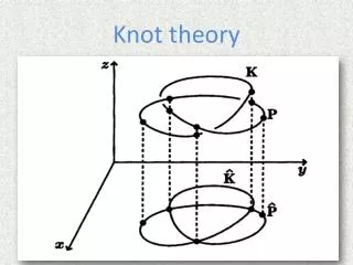
Knot Theory
Knot Theory. Whitney Sherman. Objectives. To show that the Kauffman Bracket is unchanged under each of the three Reidemeister moves. First explain the basics of knot theory. Then show you what the Reidemeister moves are, and how they affect knots.

Knot Theory
E N D
Presentation Transcript
Knot Theory Whitney Sherman
Objectives • To show that the Kauffman Bracket is unchanged under each of the three Reidemeister moves. • First explain the basics of knot theory. • Then show you what the Reidemeister moves are, and how they affect knots. • Finally, illustrate the Kauffman Bracket and it’s applications.
Questions to Consider • Given a loop, is it really knotted, or can it be untangled without having to be cut? • Given two Knots how do you tell whether the two Knots are the same or different? • Is there an effective algorithm to answer the above questions?
What is a Knot • A piece of string with a knot tied in it • Glue the ends together because it is necessary in knot theory that a knot be a continuous loop.
Deformation • If you deform a knot in the plane without cutting it, it doesn’t change.
Alternating Knot • Goes under, over, under, over…
The Unknot • The simplest knot. • An unknotted circle, or the trivial knot. • You can move from the one view of a knot to another view using a series of Reidemeister moves.
Reidemeister Moves • Reidemeister moves change the projection of the knot. • This in turn, changes the relation between crossings, but does not change the knot.
Reidemeister Moves • First: Allows us to put in/take out a twist. • Second: Allows us to either add two crossings or remove two crossings. • Third: Allows us to slide a strand of the knot from one side of a crossing to the other.
Theorem • Given two knots and , then iff you can get from to by a series of Reidemeister Moves.
Links • A set of disjoint knots. • The classic Hopf Links with two components and 10 components. • The Borremean Rings with three components.
Linking Number • The linking number is a way of measuring numerically how linked up two components are. • If there are more than two components, add up the link numbers and divide by two. Negative crossing -1 If you rotate the under-strand counterclockwise they line up Positive crossing +1 If you rotate the under-strand clockwise they line up
Example • Rotate under strand • Linking number is +1 +1 -1 +1 +1
+1 -1 -1 -1 +1 +1 What it Does For Us... • The linking number is unaffected by all three Reidemeister moves. Therefore it is an invariant of the oriented link.
Writhe • To calculate the writhe you must start with an oriented knot or link projection. • At each crossing you will have either a +1 or a -1. • The writhe is the sum of these numbers. • It is expressed as where is a link projection. 1+1-1-1=0 So the writhe of the figure eight knot is 0 +1 -1
-1 +1 +1 +1 +1 -1 -1 +1 What it Does For Us... • The writhe of a knot projection is unaffected by Reidemeister moves II and III thus becomes useful for other knot polynomials, such as the Kauffman X polynomial. -1
Kauffman Bracket in Terms of Pictures • Three Rules
To Prove Invariance • In order to show that a given polynomial is in fact knot/link invariant, it is necessary and sufficient to show that the invariant in question is unchanged under each of the three Reidemeister moves. • I.E. I need to show that the Kauffman Bracket is unchanged under each of the three Reidemeister moves.
2nd Reidemeister Move Cont. • We want the polynomials to satisfy the Reidemiester moves so, let’s find B in terms of A. • The same is done to determine C:
Kauffman Bracket • Three Rules
Regular Isotopy • This shows that the bracket polynomial is invariant under Reidemeister moves II and III i.e. is an invariant of regular isotopy. • It is not an invariant under Reidemeister I • The next task is to find a way to make it work.
Isotopy • Planar Isotopy is the motion of a diagram in the plane that preserves the graphical structure of the underlying projection. • A knot or a link is said to be Ambient isotopic to another if there is a sequence of Reidemeister moves and planar equivalences between them.
The Kauffman X Polynomial • In a type 1 Reidemeister move the Kauffman Polynomial looks like • We know • Since the writhe of the unknot is 0, then Kauffman Bracket Kauffman X Polynomial
1st Reidemeister Move • So, now the Type I move can be calculated: • Now, X(L) is invariant since it does not change with any of the Reidemeister moves.
Picture Example • Hopf Link
Another Way of Looking at the Bracket Polynomial • Labeling a crossing • Labeling a Projection
A and B Split • Crossing • A-Split • B-Split
State • The choice of how to split all n-crossings in a projection L. • Denoted: • Notice that this particular state of the trefoil contributes to the bracket polynomial of this projection
The State Model Bracket Polynomail • The bracket polynomial of a link L will now simply be the sum over all the possible states. • Denoted: • Where is the number of A-splits in S, and is the number of B-splits in S.
Advantages • To compute the bracket polynomial of the trefoil knot. • There are 3 crossings so there will be states
Applications of the Kauffman Bracket • It is hard to tell the unknot from a messy projection of it, or for that matter, any knot from a messy projection of it. • If does not equal , then can’t be the same knot as . • However, the converse is not necessarily true.
Conclusions • I have proved that the Bracket polynomial is invariant under the three Reidemeister moves.
Further Research • Knot Theory has many applications in other fields, specifically biology. • Knot theory aids in DNA research of knotted or tangled DNA.
Resources • Pictures taken from • http://www.cs.ubc.ca/nest/imager/contributions/scharein/KnotPlot.html • Other information from • The Knot Book, Colin Adams • Complexity: Knots, Colourings and Counting, D. J. A. Welsh • New Invariants in the Theory of Knots, Louis Kauffman • Jo Ellis-Monaghan
Labeling Technique for Shaded Knot/Link Projections • Begin with the shaded knot projection. • If the top strand ‘spins’ left to sweep out black then it’s a + crossing. • If the top strand ‘spins’ right then it’s a – crossing. - +
Links to Planar Graphs • Given a knot projection • Shade it so that the outside region is white/blank. • Put a vertex inside each shaded region. • Connect the regions if the shaded areas share a crossing.
Kauffman Bracket In Polynomial Terms • if is an edge corresponding to: • A negative crossing: • There exists a graph such that where and denote deletion and contraction of the edge from • A positive crossing: • There exists a graph G such that