Download
1 / 33
330 likes | 451 Views
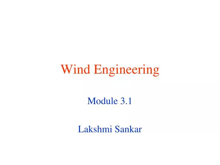
Wind Engineering. Module 3.1 Lakshmi Sankar. Recap. In module 1.1, we looked at the course objectives, deliverables, and the t-square web site. In module 1.2, we looked at the history of wind turbine technology, some terminology, and definitions.

E N D
Wind Engineering Module 3.1 Lakshmi Sankar
Recap • In module 1.1, we looked at the course objectives, deliverables, and the t-square web site. • In module 1.2, we looked at the history of wind turbine technology, some terminology, and definitions. • In module 1.3, we looked at three studies – an off-shore site, guidelines for small wind turbines, and design of utility class wind turbines. • Once module 1 is completed, you are ready to select a wind turbine anywhere in the world that you choose, and learn about the wind resources, energy needs, environmental issues, public policies, etc.
Recap, continued • In module 2, we modeled the wind turbine as an actuator disk. • We found that air starts decelerating even before it reaches the rotor disk. One half of the deceleration takes place upstream of the wind turbine, and the other half of the deceleration takes place in the space between the rotor and the far wake. • We discovered Betz limit: If wind has a velocity of V, and the turbine disk area is A, the maximum power that can be extracted is (16/27) * ½ * rho * V ^3 * A
L D L sinf Dcosf Wr f Vwind - Vinduced Use of Lift forces for Torque Production Propulsive force = L`sinf – D`cosf
Lift and Drag Forces • In module 1.2, we discussed that the net thrust force is L’sin(f) – D’ cos(f) • L’ is the lift force per unit span of the rotor section, and D’ is the drag force per unit span. • In this module, we will learn how to compute or estimate L` and D`. • In module 3.1, we will first learn some basic characteristics of airfoils. • In module 3.2, we will develop the governing equations. • In module 3.3, we will show how to solve the equations on computer using panel method to compute lift. • In module 3.4, we will discuss how the panel method is used with empirical methods to compute the viscous drag forces • In module 3.5, we will discuss how designers change the shape of the airfoils to get high L’ and low D’ at the same time.
Topics To be Studied • Airfoil Nomenclature • Lift and Drag forces • Lift, Drag and Pressure Coefficients
Uses of Airfoils • Wings • Propellers and Turbofans • Helicopter Rotors • Compressors and Turbines • Hydrofoils (wing-like devices which can lift up a boat above waterline) • Wind Turbines
Evolution of Airfoils Early Designs - Designers mistakenly believed that these airfoils with sharp leading edges will have low drag. In practice, they stalled quickly, and generated considerable drag.
Airfoil Equal amounts of thickness is added to camber in a direction normal to the camber line. Camber Line Chord Line
An Airfoil is Defined as a superposition of • Chord Line • Camber line drawn with respect to the chord line. • Thickness Distribution which is added to the camber line, normal to the camber line. • Symmetric airfoils have no camber.
Angle of Attack a V Angle of attack is defined as the angle between the freestream and the chord line. It is given the symbol a. Because modern wings have a built-in twist distribution, the angle of attack will change from root to tip. The root will, in general, have a high angle of attack. The tip will, in general, have a low (or even a negative) a.
Lift and Drag Forces acting on a Wing Section Sectional Lift, L ´ Sectional Drag, D´ V The component of aerodynamic forces normal to the freestream, per unit length of span (e.g. per foot of wing span), is called the sectional lift force, and is given the symbol L ´. The component of aerodynamic forces along the freestream, per unit length of span (e.g. per foot of wing span), is called the sectional drag force, and is given the symbol D ´.
Sectional Lift and Drag Coefficients • The sectional lift coefficient Cl is defined as: • Here c is the airfoil chord, i.e. distance between the leading edge and trailing edge, measured along the chordline. • The sectional drag force coefficient Cd is likewise defined as:
Note that... • When we are taking about an entire wing we use L, D, CL and CD to denote the forces and coefficients. • When we are dealing with just a section of the wing, we call the forces acting on that section (per unit span) L´ and D ´, and the coefficients Cl and Cd
Pressure Forces acting on the Airfoil Low Pressure High velocity High Pressure Low velocity Low Pressure High velocity High Pressure Low velocity Bernoulli’s equation says where pressure is high, velocity will be low and vice versa.
Pressure Forces acting on the Airfoil Low Pressure High velocity High Pressure Low velocity Low Pressure High velocity High Pressure Low velocity Bernoulli’s equation says where pressure is high, velocity will be low and vice versa.
Subtract off atmospheric Pressure p everywhere.Resulting Pressure Forces acting on the Airfoil Low p-p High velocity High p-p Low velocity Low p-p High velocity High p-p Low velocity The quantity p-p is called the gauge pressure. It will be negative over portions of the airfoil, especially the upper surface. This is because velocity there is high and the pressures can fall below atmospheric pressure.
Relationship between L´ and p(Continued) Divide left and right sides by We get:
Pressure Coefficient Cp From the previous slide, The left side was previously defined as the sectional lift coefficient Cl. The pressure coefficient is defined as: Thus,
Why use Cl, Cp etc.? • Why do we use “abstract” quantities such as Cl and Cp? • Why not directly use physically meaningful quantities such as Lift force, lift per unit span , pressure etc.?
The Importance of Non-Dimensional Forms Consider two geometrically similar airfoils. One is small, used in a wind tunnel. The other is large, used on an actual wing. These will operate in different environments - density, velocity. This is because high altitude conditions are not easily reproduced in wind tunnels. They will therefore have different Lift forces and pressure fields. They will have identical Cl , Cd and Cp - if they are geometrically alike - operate at identical angle of attack, Mach number and Reynolds number
The Importance of Non-Dimensional Forms In other words, a small airfoil , tested in a wind tunnel. And a large airfoil, used on an actual wing will have identical non-dimensional coefficients Cl , Cd and Cp - if they are geometrically alike - operate at identical angle of attack, Mach number and Reynolds number. This allows designers (and engineers) to build and test small scale models, and extrapolate qualitative features, but also quantitative information, from a small scale model to a full size configuration.
The geometry must be similar (i.e. scaled) between applications. The Reynolds number must be the same for the model and full scale. The Mach number must be the same for the model and full scale. Then, the behavior of non-dimensional quantities Cp, CL, CD, etc will also be the same. Once Cl, Cd etc. are found, they can be plotted for use in all applications - model or full size aircraft
Characteristics of Cl vs. a Stall Cl Slope= 2p if a is in radians. a = a0 Angle of zero lift Angle of Attack, a in degrees or radians
The angle of zero lift depends onthe camber of the airfoil Cambered airfoil Cl a = a0 Symmetric Airfoil Angle of zero lift Angle of Attack, a in degrees or radians
Mathematical Model for Cl vs. a at low angles of attack Incompressible Flow: a is in radians
Drag is caused by • Skin Friction - the air molecules try to drag the airfoil with them. This effect is due to viscosity. • Pressure Drag - The flow separates near the trailing edge, due to the shape of the body. This causes low pressures near the trailing edge compared to the leading edge. The pressure forces push the airfoil back. • Wave Drag: Shock waves form over the airfoil, converting momentum of the flow into heat. The resulting rate of change of momentum causes drag.
Skin Friction Particles away from the airfoil move unhindered. Particles near the airfoil stick to the surface, and try to slow down the nearby particles. A tug of war results - airfoil is dragged back with the flow. This region of low speed flow is called the boundary layer.
Laminar Flow This slope determines drag. Airfoil Surface Streamlines move in an orderly fashion - layer by layer. The mixing between layers is due to molecular motion. Laminar mixing takes place very slowly. Drag per unit area is proportional to the slope of the velocity profile at the wall. In laminar flow, drag is small.
Turbulent Flow Airfoil Surface Turbulent flow is highly unsteady, three-dimensional, and chaotic. It can still be viewed in a time-averaged manner. For example, at each point in the flow, we can measure velocities once every millisecond to collect 1000 samples and and average it.
“Time-Averaged” Turbulent Flow Velocity varies rapidly near the wall due to increased mixing. The slope is higher. Drag is higher.
In summary... • Laminar flows have a low drag. • Turbulent flows have a high drag. • The region where the flow changes from laminar to turbulent flow is called transition zone or transition region. • If we can postpone the transition as far back on the airfoil as we can, we will get the lowest drag. • Ideally, the entire flow should be kept laminar.