Download
1 / 19
190 likes | 373 Views
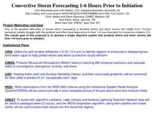
Convective Storm Forecasting 1-6 Hours Prior to Initiation. Dan Lindsey (STAR/RAMMB) John Mecikalski (UAH) Chris Velden (CIMSS) Bob Rabin (NSSL ) Brian Vant-Hull (CREST ) Louie Grasso (CIRA) John Walker (UAH) Lori Schultz (UAH) Steve Wanzong (CIMSS).

E N D
Convective Storm Forecasting 1-6 Hours Prior to Initiation Dan Lindsey (STAR/RAMMB) John Mecikalski (UAH) Chris Velden (CIMSS) Bob Rabin (NSSL) Brian Vant-Hull (CREST) Louie Grasso (CIRA) John Walker (UAH) Lori Schultz (UAH) Steve Wanzong (CIMSS) This work is supported by GOES-R Risk Reduction
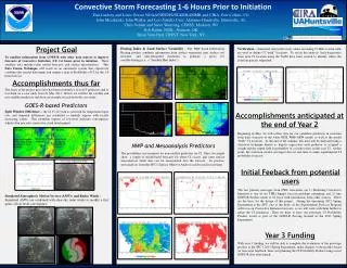
Motivation • Predicting where and when convection will form continues to be one of the biggest problems facing forecasters • Numerical models, especially high resolution (<=4 km) models, do a pretty good job with predicting convection, but rarely correctly pinpoint the time and location of CI • This project seeks to investigate various uses of GOES-R ABI data to improve short-term (1-6 hour prior) Convective Initiation (CI) forecasts
Methodology • We’re using 4-km NSSL WRF ARW model output to simulate GOES-R ABI data, then looking at the relationship between certain satellite and environmental parameters with CI • Possible CI predictors include: • 10.35-12.3 µm split window difference • Low-level convergence derived from mesoscale Atmospheric Motion Vectors (AMVs) • Horizontal gradients in sensible heating • Low-level Convergence derived from clear-sky WSR-88D radar winds • We’re also looking at MSG/SEVIRI data as a proxy for ABI whenever possible
Convective Initiation and Sensible Heating Gradients CI occurring on sensible heating (SH) in humid Southeast U.S. • CI occurs along gradients in sensible heating if synoptic scale forcing is weak (Walker et al. 2009). • Yet, many other factors dictate CI on a given day, at a given time and location. • SH gradients cannot really be used alone in CI nowcasting.
Premise for using SH gradients lies in the ability to discern cites and other geographical features. Cities “heat islands” are known to cause CI over and downwind. Gradients in sensible heating lead to the development of non-classical mesoscale circulations, which can help weaken and break a capping inversion, especially when larger scale convergent forcing is weak. Indianapolis Indianapolis Memphis Atlanta Mississippi Delta Birmingham Black belt
Simulated Atmospheric Motion Vectors (AMVs) and Radar Winds AMVs are derived from WRF model 4km simulated IR and VIS images at 5-min. intervals (proxy for GOES-R capability), and combined with clear-sky radar winds to modify a model analysis of low-level convergence prior to a convective event in OK/KS on 21 May (2011). Top Left: Low-level model winds and contoured convergence field; Top Right: Low-level simulated AMVs and resultant modified convergence field ; Bottom Left: AMVs plus radar-derived wind vectors over OK, and modified convergence analysis; Bottom Right: Sample Doppler radial velocity field used to obtain the radar wind field.
Simulated Atmospheric Motion Vectors (AMVs) and Radar Winds The example loop below shows the model-computed 1-km divergence field (so the negative values show convergence), and the Convective Initiation locations are shown with small black contours. Note the convergence signature in central Oklahoma and northern Texas that preceded CI. A product using AMVs and Radar-derived winds could potentially capture these convergence signatures.
CI Hits and Back Trajectory Analysis Simulated radar reflectivity values exceeding 35 dBZ at 4-km AGL are used to define CI “truth” locations. To aid in the analysis, back-trajectories from each CI location using the NAM have been created to identify where the cloud air parcels originated.
10.35-12.3 µm “Split Window Difference” • It’s long been known that the split window difference provides information about atmospheric water vapor content • Radiation at 12.3 µm is preferentially absorbed and re-emitted by water vapor, so deeper moisture generally results is a larger positive 10.35 – 12.3 µm difference • The two primary determinants for the split window difference are: • Amount and depth of water vapor (WV), especially at low levels • The temperature lapse rate. Steeper (more unstable) low-level lapse rates (LR) result in larger positive differences • So the brightness temperature difference (BTD) can be parameterized by: • BTD ~ WV * LR
Example: 20 May 2013 Data from the 4-km NSSL WRF-ARW model is used to simulate the GOES-R ABI bands 10.35 - 12.3 µm – 15:00 to 00:00 UTC ABI 10.35 µm – 15:00 to 00:00 UTC
Example: 20 May 2013 10.35 - 12.3 µm – 18:00 UTC Sfc-700mb specific humidity * Lapse Rate 18:00 UTC BTD ~ WV * LR
Example: 20 May 2013 10.35 - 12.3 µm – 18:00 UTC Sfc-700mb specific humidity * Lapse Rate
Example: 20 May 2013 10.35 - 12.3 µm – 18:00 UTC
Example: 20 May 2013 Vertical cross-section 10.35 - 12.3 µm – 18:00 UTC
Example: 20 May 2013 Specific Humidity (kg/kg) and 10.35-12.3 µm (white contour, right vertical axis)
Example: 20 May 2013 BTD ~ WV * LR WV ~ BTD/LR so if we measure the BTD and we know the lapse rate, the low-level water vapor can be estimated
Example: 20 May 2013 “Normalized” split window difference: (10.35 – 12.3 µm) / sfc-700mb Lapse Rate – 18:00 UTC Sfc-700 mb Specific Humidity and surface winds – 18:00 UTC • Note the spatial similarity between these two maps; this shows that the normalized split window difference is essentially a low level water vapor retrieval
Example: 20 May 2013 “Normalized” split window difference: (10.35 – 12.3 µm) / sfc-700mb Lapse Rate 10.35 - 12.3 µm – 17:00 to 22:00 UTC • *However*, the unaltered split window difference better identifies where convective clouds and storms are likely to form, because it maximizes where deep moisture overlaps with steep lapse rates
Conclusions • The GOES-R based potential CI predictors we looked at each are useful only under certain (different) environmental conditions, so a single product using all of them simultaneously is not feasible • However, each predictor alone provides value in certain situations • Sensible heating gradients may point to CI locations under benign synoptic conditions, such as in the southeast U.S. during mid-summer • When low-level trackable clouds are present, mesoscale atmospheric motion vectors may be used to derive low-level winds, which in turn provide information on convergence • Clear sky radar echoes, when enough scatterers (bugs, etc.) exist, can also be used to derive low-level convergence • The 10.35 – 12.3 µm product works well under clear sky conditions to identify regions of low-level pooling of moisture and often convective cloud formation. The difference itself may be more useful than an actual moisture retrieval because it highlights areas that have both deep moisture and steep low-level lapse rates • After GOES-R is launched and the real data is flowing, these ideas can be used to develop actual products to aid in CI forecasting