Download
1 / 65
670 likes | 780 Views
Electrical Resistance Imaging of Binary Mixtures. NU-CNU Workshop 9 th of July 2008, Nagasaki University. Kyung-Youn KIM* and Sin KIM ** * kyungyk@cheju.ac.kr , Professor of Department of Electronic Engineering

E N D
Electrical Resistance Imaging of Binary Mixtures NU-CNU Workshop9th of July 2008, Nagasaki University • Kyung-Youn KIM* and Sin KIM ** • * kyungyk@cheju.ac.kr, Professor of Department of Electronic Engineering • ** sinkim@cheju.ac.kr, Professor of Department of Nuclear and Energy • Engineering • Cheju National University, KOREA
Contents • Introduction • Basic Concept of ERT (Electrical Resistance Tomography) • Related Physical Laws • Governing Equation • Mathematical Models for ERT • Summary of ERT Problem • Forward Problem • Inverse Problem • Some Issues in ERT • Ill-Posedness and Regularization • Inverse Crime • Data Collection Methods and Current Patterns • Static vs. Dynamic Imaging • Internal Structures and Masking Effect
Novel Algorithms for Binary Mixtures • Mesh Grouping Algorithm • Boundary Estimation • Front Point Estimation • Particle Concentration Imaging • Further Studies
Introduction Basic Concept of ERT • Electrical Resistance Tomography (ERT) is an imaging modality in which the internal electrical conductivity distribution is reconstructed based on the imposed currents and the measured voltages at the electrodes placed on the surface.
Characteristics • Non-Intrusive measurement • Poor spatial resolution, but high temporal resolution (cf. CT, MRI) • No health problem (cf. X-ray, CT) • Inexpensive hardware, but sophisticated software • Applications • Medical imaging, medical diagnosis (apnea, osteoporosis) • Process tomography • Geological applications (hydrology, location of oar bodies)
Motives of the Introduction of ERT to Binary Mixtures (e.g. Two-Phase Flows) • Distinct conductivities (e.g. water and vapor) • Fast transient (cf. CT, MRI) • Multi-dimensional (cf. conductivity probe, optical probe) • Complex flow geometry, e.g. rod bundles • Non-intrusive technique • Application to Two-Phase Flow • Visualization or monitoring of two-phase flow fields • Identification of flow regime • Heat transfer and hydrodynamic characteristics are dependent on the flow regime. • Measurement of void fraction • Void fraction is the most important variable in the analysis of two-phase flows.
Related Physical Laws • A quantitative description of the current flow within an arbitrary body • Faraday’s law of induction: Curl E = - B/t where E = electric field, B = magnetic induction • Extended Ampère’s law: Curl H = J + D/t where H = magnetic field, J = current density vector, D = electric displacement • Current density: J = J0 + JS where J0 = Ohmic current, JS = current source • D = eE, B = mH, J0 = sE in linear isotropic medium where e = permittivity, m = permeability, s = conductivity • If the injected currents are time-harmonic with frequency w E = E0exp(iwt), B = B0exp(iwt) • Curl E = - iwmH, Curl H = (s+iwe)E + JS or Div (iwmH) = 0, Div (s+iwe)E = - Div JS • Description of electric field: E = - Grad u - A/t where u = electric potential, A = magnetic vector potential (B = Curl A)
Governing Equation • Governing Equation • If the effect of magnetic induction is neglected ( wmsLc(1+we/s) << 1 ) E = - Grad u eg) water: m ~ 10-6Vs/Am, e ~ 10-9C2/Nm2, w/2p ~ 10kHz, Lc~ 1m wmsLc(1+we/s) ~ 0.001 << 1 for s ~ 0.1/Wm, Div (s+iwe) Grad u = 0 • Boundary Conditions Div sE dS = - Div JS dS or su/n = j where j = injected current density • we/s << 1 : electrical resistance tomography (ERT) • or electrical impedance tomography (EIT) • we/s >> 1 : electrical capacitance tomography (ECT)
Electrode Model • Continuum model: • Neglect the effect of electrode • Overestimate the resistivity as much as 25% • Gap model: • Improve continuum model • Neglect the shunting effect • Still overestimate the resistivity • Shunt mode: • Neglect the contact impedance between the electrode and the object • Underestimate the resistivity • Complete electrode model: • Consider both the shunting effect and the contact impedance
Mathematical Models for ERT Summary of ERT Problem • The forward problem calculates the boundary voltages by using the assumed resistivity distribution (e.g. bubble distribution). • The inverse problem reconstructs the resistivity distribution minimizing the difference between the measured and the calculated boundary voltages.
Forward Problem el: l-th electrode Il : current at the l-th electrode L : # of electrodes Ul : voltage at the l-th electrode u : voltage zl : contact impedance :resistivity • Governing Equations • Complete Electrode Model • Consider contact impedance between the object and the electrode • Constraints to Ensure the Uniqueness of the Solution (1) in (2) l = 1, 2, , L (3) on on el, l = 1, 2, , L (4) (5)
Finite Element Formulation • The resistivity inside a finite element is assumed to be constant, so the number of finite element meshes will be the number of unknowns. • A set of current patterns imposed through the electrodes and induced voltages is required to obtain the resistivity distribution in the inverse problem. • The final discretized equation will be a linear system of equations of • Y : stiffness matrix (N+L-1)×(N+L-1) • u : voltage matrix (N+L-1)×P • c : current matrix (N+L-1)×P • N : # of nodes • L : # of electrodes • P : # of current patterns (6) Typical mesh structure
Inverse Problem • Find the resistivity distribution minimizing the difference between the measured voltages V and the calculated voltages U with the assumed r. • Conventional Gauss-Newton Method to Find r • Minimal point : • Linearization about ri: • Hessian matrix : • U// is known to be relatively small if the initial guess is close to minimum and very difficult to calculate, so it is often neglected. • Due to high ill-conditioning, regularization is required. • Resistivity update : (7) (8) (9) (10) (11)
Some Issues in ERT Ill-Posedness and Regularization • Well-Posed Problem if Its Solution • Exists • Is unique • Depends continuously on the data • Ill-Posedness is Typical in Inverse Problems. • In ERT inverse problem, the conductivity depends on the ERT data (injected currents and measured voltages) in a very weak way. • A small change in ERT data may cause a large change in the conductivity distribution. • The response may be saturated above a certain value of resistivity contrast.
Regularization is Required to Mitigate the Ill-Posedness. • Generalized Tikhonov regularization R : regularization matrix a : regularization parameter • The regularization matrix takes the prior information into account. • If the solution is bounded but fluctuating, • If the solution is smooth, • If the internal structures and their resistivity are known, where S is the extraction matrix to pick up the meshes belonging to the known internal structures and r* is the known resistivity. • The regularization parameter controls the relative weighting to the prior information. • Resistivity update: (12) (13)
Inverse Crime • In numerical experiments, if the forward and the inverse mesh structures are same numerical errors may be cancelled out inadvertently. • The forward and the inverse mesh structures should be different from each other. Fig. FEM mesh for forward problem and inverse problem
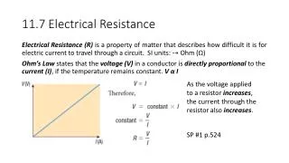
Data Collection Methods and Current Patterns • There are numerous ways in which the current-injecting electrodes are chosen. • The sensitivity depends on the data collection method. • Sensitivity is defined as a fractional change in voltage for a fractional change in conductivity contrast. where the conductivity contrast • Data collection methods • Neighboring method: good sensitivity at the periphery • Opposite method: good sensitivity at the center • Multi-reference method: simultaneous injection • Adaptive method (14)
Trigonometric current pattern where • The best current pattern to distinguish a central circular inhomogeneity • But, needs as many current generators as there are electrodes and complicated measurement system
Static vs. Dynamic Imaging • Static Imaging • Resistivity distribution is assumed to be stationary during the time required to obtain a full set of current-voltage data. (stationary or slow transient) • Gauss-Newton algorithm and its variations • Applications: medical imaging, geological imaging • Dynamic Imaging • Resistivity distribution changes within the time taken to acquire a full set of measurement data. (fast transient) • ERT problem is considered as a state estimation problem. • Kalman filter and its variations, target tracking algorithms • Applications: process tomography, visualization of two-phase flows
State Equation: Measurement Equation: • State Estimation Approach (Kalman Filter Approach) where k time index, Fk state transition matrix, wk process noise, vk measurement noise • State transition matrix: usually unknown so “random walk model” is adopted • Linearization about • LKF (Linearized Kalman Filter) • Linearization about the initial distribution • EKF (Extended Kalman Filter) • Linearization about the estimate based on (k-1)-th step (15) (16)
Time Update Measurement Update (17-1) (17-4) (17-2) (17-5) (17-3) • Recursive Equation where error covariance matrices pseudo-measurement pseudo-measurement matrix
Case 1 1~8 steps 9~16 steps True LKF EKF True LKF EKF
25~31 steps 17~24 steps True LKF EKF GN True LKF EKF
Case 2 1~8 steps 9~16 steps True LKF EKF True LKF EKF
25~31 steps 17~24 steps True LKF EKF GN True LKF EKF
Effect of Current Pattern EKFtri1 trigonometric, 1st pattern EKFtri2 trigonometric, up to 2nd patternEKFtri4 trigonometric, up to 4th pattern EKFtriAll trigonometric, all patterns EKFadj1 adjacent EKFadj2 adjacent, 90deg rotation EKFopp opposite 1 2 3 4 target EKFtri1 EKFtri2 EKFtri4 EKFtriAll EKFadj1 EKFadj2 EKFopp1
5 6 7 8 target EKFtri1 EKFtri2 EKFtri4 EKFtriAll EKFadj1 EKFadj2 EKFopp1
9 10 11 12 target EKFtri1 EKFtri2 EKFtri4 EKFtriAll EKFadj1 EKFadj2 EKFopp1
13 14 15 16 target EKFtri1 EKFtri2 EKFtri4 EKFtriAll EKFadj1 EKFadj2 EKFopp1
17 18 19 20 target EKFtri1 EKFtri2 EKFtri4 EKFtriAll EKFadj1 EKFadj2 EKFopp2
21 22 23 24 target EKFtri1 EKFtri2 EKFtri4 EKFtriAll EKFadj1 EKFadj2 EKFopp2 mn=3e-3 mn=2e-3
25 26 27 28 target EKFtri1 EKFtri2 EKFtri4 EKFtriAll EKFadj1 EKFadj2 EKFopp2 mn=3e-3 mn=2e-3
29 30 31 GN target EKFtri1 EKFtri2 EKFtri4 EKFtriAll EKFadj1 EKFadj2 EKFopp2
EKFtri1 blue EKFtri2 redEKFtri4 magenta EKFtriAll green EKFadj1 blueEKFadj2 red EKFopp magenta
Internal Structures and Masking Effect • Where high resistive target is near conductive internal structure (e.g. conductive rods), most electrical current flows through the conductive region and the sensitivity of the target is degraded. • The degradation due to the masking effect will be significant for high conductivity contrast cases. • Two ways to get around the masking effect • Use of prior information on the internal structure (geometry and conductivity) • Use of internal electrodes Fig. Known internal structure Fig. Internal electrodes
true true unknown S&R known S&R IE Fig. Reconstructed images of two-phase flows in rod bundles
true true unknown S&R known S&R IE Fig. Reconstructed images of two-phase flows in rod bundles
I III II j k0 k1 k2 k3 Novel Algorithms for Binary Mixtures Mesh Grouping Algorithm • The conventional Newton-type iterations cannot improve the reconstruction image further after a certain number of iterations due to the ill-posedness of the problem. • In binary-mixture systems like two-phase flows, there are only two resistivity values. • Sorted resistivity values in an ideal case • Group I : continuous group (e.g. water) • Group III : dispersed group (e.g. bubble) • Group II : temporary group (meshes crossing phase boundaries) • ki : element index to specify group boundary • According to the resistivity value and the threshold, each mesh is classified into one of 3 groups.
Find to minimize the following functional • In this k0=1 and k3 = M • The number of unknowns will be reduced. (M -> k2-k1+2) • The sensitivity will be enhanced. • Note that the objective functional is not analytical and the derivatives cannot be calculated. • Genetic algorithm would be a good choice to solve the problem. • Mis-Grouping may occur and it degrades the convergence significantly. • Alternately apply grouping and ungrouping (e.g. Do ungrouping every 5 iterations with grouped meshes) (18)
Construction of grouping matrix • Cont or DispGroup (Group I or III) where 1’s are located at the columns where the elements are grouped into the i-th group, i=I or III. • TempGroup (Group II) where 1’s are located at the i-th row (original element index) and j-th column (element index in the sorted) • Modified Update Equation (19)
Fig. Resistivity distribution before and after the 1st grouping
Image Reconstruction with Experimental Data True image Conventional algorithm Mesh grouping
Boundary Estimation • In the application of ERT to the imaging of two phase flows, the conductivity of each phase can be known a priori and the unknown would be the phase boundary. • Limitations of conventional algorithms in the estimation of phase boundary • Meshes crossing the phase boundaries • Extremely fine meshes for better approximation • Tremendous computational burden
Consider the inverse problem to find the phase boundary directly, not the conductivity distribution. • Representation of the phase boundary with truncated Fourier series • In two phase flows, the boundary shape is not complex. It would be circular or elliptic and Nq = 3 would enough. • Unknowns: conductivity values s -> Fourier coefficients g • g can be estimated with using the conventional Newton-type algorithm. • At every iteration, remeshing or mesh decomposition is required.
Cl(s) ATG ,TG s2 s1 ABG ,BG Fig. Remeshing Fig. Mesh decomposition
Image Reconstruction with Experimental Data True image Conventional algorithm Boundary estimation
Boundary Estimation with Prior Information from Newton-type Solution • Number of targets should be given a priori, but maybe unknown. • Conventional Newton-type algorithm can give information (number of targets, size, location) even after a single iteration.