Download
1 / 52
520 likes | 655 Views
Lagrangian tracer transport models: Measuring concentrations, assessing emissions Formulation Adjoint Mass Conservation and other complications. S. C. Wofsy, Harvard University, 25 April 2009 (1) Particle dispersion models;

E N D
Lagrangian tracer transport models:Measuring concentrations, assessing emissions Formulation Adjoint Mass Conservation and other complications • S. C. Wofsy, Harvard University, 25 April 2009 • (1) Particle dispersion models; • Adjoint implementation at Harvard: Stochastic Time-Inverted Lagrangian Transport (STILT) Model; • Application to assessment of sources of greenhouse gases to the atmosphere.
GV aircraft approaches the terminator over the Alaska range in January, 2009, in HIPPO_1 experiment to define transport rates and global sources of greenhouse gases
Global and regional studies of CO2 , other greenhouse gases, ozone destroying species, etc, use observations of concentrations at the ground, and from aircraft and satellites, to infer emission rates from surface sources.An inverse problem. Why do we want to know? • Emissions of these gases drive changes in radiative forcing, ozone loss, atmospheric chemistry • Processes regulating emissions, and overall budgets are much less certain than needed to predict future atmospheric composition • Natural vs. human—caused balances is debated • Future monetization of CO2 emissions requires verification of source reductions
NOAA Greenhouse Gas records 55% of annual emissions
Basic Lagrangian Equation: Trajectories The advection of a particle or puff is computed from the average of the three-dimensional velocity vectors for the initial-position P(t) and the first-guess position P'(t+∆t). The velocity vectors are typically linearly interpolated in both space and time. The first guess is P'(t+∆t) = P(t) + V(P,t) ∆t and the final position is P(t+∆t) = P(t) + 0.5 [ V(P,t) + V(P',t+∆t) ] ∆t, If V is the mean wind vector from an assimilated meteorological field, the equation provides a trajectory model. It is fully reversible in time, because particles (“air parcels”) do not spread. Trajectory models cannot compute concentrations because the particles have zero measure.
Puff and Dispersion Models Puff model: the source releases pollutant puffs at regular intervals. Each puff is advected according to the trajectory of its center of mass, as it expands (both horizontally and vertically) to simulate dispersion in a turbulent atmosphere. Useful for short term simulations. Lagrangian particle dispersion model: the source is simulated by releasing many particles at the same time. A random component to the motion is added at each step according to atmospheric turbulence ( unresolved motions). Useful for longer term simulations. Both require that stability and mixing coefficients be computed from meteorological data.
Lagrangian approach to atmospheric chemistry models : Particle Dispersion Modeling • Air parcels are represented by particles advected with the mean wind plus stochastic velocities that simulate turbulent transport, convection, and other unresolved/"non-conservative" motions of the atmosphere. • Particle positions are resolved to arbitrary accuracy, reducing grid-averaging errors such as representation error (for observations) and source spreading (for emissions). • Particles may be followed backwards in time, providing a direct adjoint model. Lagrangian particle dispersion models, and the analogous puff dispersion models, look superficially like trajectory models (same basic equation), but there are fundamental differences. Reversibility follows a statistical criterion.
Time reversal and the advection-diffusion equation for mass transport nc/t = (Unc) + F Time reversal velocity reversal: t´ -t ; U´ - U; F = <U'c'>, does not change sign ! Diffusion does not reverse—puffs or ensembles of particles expand, forward or backward in time! The direction of the velocity in a random walk varies randomly, thus u' -u changes nothing.
Receptor-oriented model: time-inverted (adjoint) model Dispersion Random walk X2/t n2 steps to move nDL
Receptor-oriented model: time-inverted (adjoint) model Particles tell where air is arriving from and link observations with upstream sources/sinks
Backward Lagrangian transport (x, y, z) receptor (xi’,yi’,zi’) source
Forward = Backward? (x, y, z) receptor (xi’,yi’,zi’) source Backward forward
STILT(Stochastic Time Inverted Lagrangian Transport Model) Receptor location stochastic (turbulent) advection mean advection u’depends on: 1) TL (decorrelation timescale) 2) sw (fluctuations in turbulent velocity) • Based on HYSPLIT (Hybrid Single Particle Lagrangian Integrated Trajectory) model code [Draxler and Hess, 1998] • Driven by ETA, AVN (forecasts) or EDAS, GDAS, NGM (assimilations) • Improved turbulence parameterization • TLw (vertical) and sw after Hanna [1982] • reflection/transmission scheme at interfaces between high and low turbulence after Thomson [1997] (“off-line” model)
Framework: Lagrangian Particle Dispersion Model Framework: A particle ensemble is released at the receptor and transported backward in time, tracking air parcels that arrive (in the forward-time sense) at the receptor at a given time. The density of STILT particles is used to calculate the influence function I(xr,tr|x,t) and the footprint f(xr, tr| x,t). I(xr,tr|x,t) and f(xr, tr| x,t) link concentration measurements at the receptor, C(xr, tr), to the sum of all upstream contributions: C(xr, tr) = Units: C is in ppm; I is vol-1 (density); S is ppm s-1;
Influence Function, I I(xr,tr|x,t) is represented by the density r(xr,tr|x,t) of particles at (x,t) which were transported backward in time from (xr,tr), normalized by the total particle number Ntot: The fields of I(xr,tr|x,t) and S(x, t), continuous in space and time, are in practice resolved only at finite resolution with a discrete volume (x,y,z) and finite time interval (t). Integrating over the finite volume and time elements to get the time/volume integrated I:
Source-receptor matrix elements in I (tr, xr, yr, zr | ts, xs, ys, zs ) (finite small volume, time interval…) The time- and volume-integrated influence function is simply quantified by tallying Dtp,m,i,j,k, the total amount of time each particle p spends in a volume element i,j,k over timestep m. The source-receptor matrix elements that link sources at finite temporal and spatial resolutions directly to receptor concentrations is: I (m´, i ´, j ´, k ´ | m, i, j, k ) /(DV Dt) Model should run equally well forwards or backwards… now we should check it!
Representing Surface Sources; mass conservation (Part 1) F is surface flux (e.g. mmole m-2 s-1), h a near-surface mixing depth (m), r the mean density of dry air in h (kg m-3), mairthe molecular mass of dry air (kg mole-1), giving S in ppm s-1. Particles are effectively tagged with a mole fraction of pollutant, and the mole fraction is conserved as the particle is transported to different pressure levels. Since S is defined consistently in the interior or at the boundary, and each receptor is at a single pressure, particles are counted with the correct weight (mass is conserved) regardless of where they are emitted or observed. _
Footprint function, f: surface influence S(x,t) is integrated over discrete volume and time elements, defining the footprint function, f : In our application, f(xr, tr| xi, yj, tm) is in units of [ppm/(mmole/m2/s)], i.e. given a unit surface flux of 1 mmole/m2/s at (xi, yj, tm) persisting over a time interval t, f(xr, tr| xi, yj, tm) is the concentration change DC in ppm at the receptor.
Detailed Linkage between Observation and Upstream Sources/Sinks (“Footprint”) from STILT Footprint of Vertical Profile over WLEF from LT1600 Particle Release on June 8th, 1999 -12 hrs -6 hrs -24 hrs log10(footprint) log10[ppmv/(mmole/m2/s)]
Physical Requirements for Realistic Simulation of Source-Receptor Relationships • Simulations of transport and upstream influence by particle models must satisfy the following criteria: • maintenance of an initially well-mixed state • simulation of the close interaction between wind shear and vertical turbulence • high temporal resolution to resolve the decay in the autocorrelation of u' • consistent representation of particles as air parcels of equal mass in both the mean and turbulent transport components of the model.
Turbulent transport: 1st order Markov process Hanna [1979] showed from Eulerian and Lagrangian measurements that a Markov assumption is reasonable, i.e. that the particle velocity vector u can be decomposed into a mean component and a turbulent component u', with the turbulent component following the relation: u' (t+Dt)=R(Dt)u'(t)+u'' (t) u''is a random vector, R an autocorrelation coefficient: R(Dt) = exp(–Dt/TLi), where TLi is the Lagrangian time scale (decorrelation time) (i=u: horizontal; i=w: vertical). The random velocity u'' is: u'' = l[1-R2(Dt)]1/2 with ldrawn from a Gaussian distribution, and standard deviation si, isderived from the meteorological field (e.g. from TKE, or mixed-layer height+surface fluxes of heat, momentum).
Beware of Looking Under the Hood:Issues Addressed in Time-Reversibility Comparisons In this house we obey the Laws of Thermodynamics! -- Homer Simpson • Wind coming out of ground • Failure to incorporate vertical density gradients • Outliers from random Gaussian generator • Operator splitting • Particles trapped in low-turbulence regions
Problem: Particles become trapped in low-turbulence regions!(spurious entropy loss) altitude Particles accumulate here. This problem is closely analogous to the problem of detailed balance in the kinetic theory of gases. sw more turbulent
Satisfying the Well-Mixed Criterionby Treating Turbulence Profiles as Separate Layers z altitude sw sw
Problem: Particles become trapped in regions of spurious mass loss! Actual simulation of particle densities for a set of winds from EDAS-80. Violates 2nd law of Thermodynamics…
Backward- vs Forward-time Comparison NGM Mass-violating Winds for one starting time orthogonal regression 1st order mass correction Particle Density in Source Box [#/km3] (Backward) 1:1 Line Particle Density in Receptor Box [#/km3] (Forward)
source receptor
source creation of mass receptor
source destruction of mass receptor
Implications of Mass Violation • Affects lots of atmospheric models, especially ‘off-line’ models • Careful attention needed in using wind fields from other models! • Forward-time not necessarily better than backward-time results • Resulting time-irreversibility may be an issue for ‘adjoint’ models as well
Backward- vs Forward-time ComparisonMass-Conserving Winds Mass-conserving, Simplified Winds orthogonal regression 1:1 Line (Backward) Particle Density in Source Box [#/km3] slope=0.98±0.03 R2=0.97 Particle Density in Receptor Box [#/km3] (Forward)
Applications of STILT • CH4, N2O, CO at ground stations, from aircraft. • CO2 sources and sinks globally
100 cumulative CO from emissions [ppb] 50 0 10 9 100 200 date (Aug. 1999) 8 model time back [h] 300 7 250 obs CO ppb 200 150 7 8 9 10 Date (August 1999) Quantifying Anthropogenic Combustion Contributions to C Budget Example: CO at Harvard Forest, 1999. Courtesy C. Gerbig, J. Lin log influenceppm/(mmol-2s-1) log influenceppm/(mmol-2s-1)
STILT shows that: Accurate measurements from a single tall tower "cover" a remarkably large area. log10 Influence: ppm per unit flux (mmole m-2s-1) at WLEF 396 m Scott M. Miller (2008) STILT
Methane and Nitrous Oxidein North America: Using an LPDM to Constrain Emissions Eric Kort kort@fas.harvard.edu Non-CO2 Workshop October 23, 2008
Case Study- COBRA-NA 2003 • ~300 flasks measured @ NOAA/Boulder, UND Citation II, 23 May to 28 June 2003
1600 1700 1800 1900 2000 CH4 0 50 100 150 200 250 300 Flask number June 16, 2003 36.72N,96.94W 609 m AGL WRF LPDM Model: STILT Emissions: EDGAR-2000 Met fields: WRF (AER, 35 km, LPDM outputs, Grell-2)
Footprint * Prior Emission Field (EDGAR) * Result = Enhancement of gas at measurement point due to source
Prior Emissions Fields • Nitrous Oxide • Anthropogenic- EDGAR32FT2000 • Anthropogenic & Biogenic- GEIA • Methane • Anthropogenic- EDGAR32FT2000 • Biogenic- Jed Kaplan wetland inventory FIRES
Results- Methane Slope: 0.924 ± 0.13 Scaling Factor: 1.08 ± 0.15 Note: Prior Emissions Field EDGAR32FT 2000 & JK wetland
STILT LPDM provides directly applicable error estimates for Bayesian inverse. 1760 1780 1800 1820 1840 1860 PDF for model CH4 concentrations for 100 particles from one receptor: Mean: 1790 ppb; 2 = 38 ppbv CH4 (ppb) (model, each particle) Measurement Error: Atmospheric Variability in a correlation length (170 km) derived from CO measurement & CO:CH4 ratio:2 = 23 ppbv
WRF/STILT/EDGAR model vs data, with gray and green. Errors used in fitting are + 38 ppbv for the model, and + 23 ppbv for the measurements Slope = 0.9 slope = 0.1 EDGAR—2000 confirmed ±10% for CH4 ! This result pertains to urban-industrial sources, which dominate the flight region
N2O Observed vs Model (EDGAR—2000 ) COBRA-2003 Model STILT/ N2O (ppbv) US sources of N2O are ~2.5x higher than EDGAR Kort et al., 2008 Observed N2O (ppbv)
CO, 3! EPA Inventory 3!
Summary—Lagrangian particle dispersion models for source assessment • Lagrangian particle dispersion models provide powerful tools to utilize atmospheric observations to study sources and sinks of atmospheric greenhouse gases. • Their unique capability to run forward and backward in a consistent numerical framework permits checks on model transport not available any other way. • Considerable effort is needed to ensure proper formulation of this type of model. Rigorously mass-conserving wind fields are required. • Applications to aircraft measurements over North America reveal important aspects of greenhouse gas emissions on continental scale.