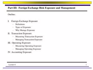
Foreign Exchange Exposure
Foreign Exchange Exposure. Foreign Exchange Exposure. How do we measure the exchange rate risk facing an MNC? Foreign exchange exposure is defined as the degree to which a company is affected by exchange rate changes.

Foreign Exchange Exposure
E N D
Presentation Transcript
Foreign Exchange Exposure How do we measure the exchange rate risk facing an MNC? Foreign exchange exposure is defined as the degree to which a company is affected by exchange rate changes. The magnitude of the gain or loss that results from a particular exchange rate change is: FX Gain (Loss) = [ St+n - St ] [ Exposure ] Exposure is expressed in units of the underlying host currency, the exchange rate is the price of the host currency in units of home currency (i.e. $/FC), and hence the exchange rate gain/loss is in home currency units.
Foreign Exchange Exposure • There are three important kinds of exposure: • Translation Exposure (or Accounting Exposure) • Transaction Exposure (or Contractual Exposure) • Economic Exposure (or Operating Exposure) • Although we shall see that economic exposure is most important measure, firms are concerned with all three. • Hence, each measure is worth understanding.
Translation Exposure Translation exposure is relevant to the preparation of the parent company’s financial statements, where a firm’s foreign currency-denominated accounts on the balance sheet are affected by exchange rate changes. Translation exposure is currently defined for U.S. firms by the Financial Accounting Standards Board (FASB) in Statement No. 52 - called FASB-52, which quantifies translation exposure as the difference between total assets and total liabilities. Hence, to determine the foreign exchange gain or loss, the net asset position (assets minus liabilities) is used as the measurement of exposure.
Summary of Translation Exposure Step 1: Determine functional currency
Summary of Translation Exposure Step 1: Determine functional currency Host currency Step 2: Translate using current method - recording gains/losses in the balance sheet as unrealized.
Summary of Translation Exposure Step 1: Determine functional currency Host currency Home currency Step 2: Translate using current method - recording gains/losses in the balance sheet as unrealized. Step 2: Translate using temporal method - recording gains/losses in the income statement as realized.
Summary of Translation Exposure Step 1: Determine functional currency Host currency Home currency Step 2: Translate using current method - recording gains/losses in the balance sheet as unrealized. Step 2: Translate using temporal method - recording gains/losses in the income statement as realized. Step 3: Consolidate into parent company’s financial statements.
Transaction Exposure Transaction exposure is the degree to which cash and transactions denominated in a foreign currency and already entered into for settlement at a future date are affected by exchange rate changes. Transaction exposure measures net cash and known cash inflows against known cash outflows.
Economic Exposure Translation (or accounting) measures of exposure are based on changes in book values of foreign currency assets and liabilities. Since the value of a firm is equal to the present value of future cash flows, translation exposure - while necessary for consolidating subsidiary and parent financial statements - usually has no bearing on the firm’s valuation. Economic exposure measures the effects of exchange rate changes on a firm’s operating cash flows and, thereby, its market value.
Economic Exposure Economic exposure integrates three key aspects of exchange rate risk: Cash flow exposure: the impact of exchange rate changes on the future operations of a firm - how costs and revenues denominated in different currencies fluctuate. 2. Net worth exposure: the impact of exchange rate changes on the market values of fixed assets and inventory. 3. Real exchange risk: accounting for exchange rate changes that result from differences in national inflation rates.
Economic Exposure • Why real exchange rate changes? • Relative price changes ultimately determine a firm’s long-run exposure to currency change. • Currency changes - particularly those of high-inflation currencies - are usually preceded by or accompanied by changes in relative price levels between two countries. • Hence, it is impossible to determine exposure to a given currency without considering simultaneously the offsetting effects of these price changes. • Alternatively, exchange rates often affect firms most severely when the nominal exchange rate does not move at all - when relative price changes are not being offset by exchange rate adjustments.
Cash Flow Exposure Cash flow exposure evaluates the ongoing cash flows of the firm. These cash flows are evaluated from a real standpoint - they are adjusted for inflation. Therefore, cash flow exposure (also know as income statement exposure or real operating exposure) is the extent to which a firm’s real revenues and expenses are affected by exchange rate changes. The sectors of the economy in which the firm operates, the sources of the firm’s inputs, and fluctuations in real exchange rates delineate the firm’s true economic exposure.
Net Worth Exposure The second component of economic exposure is net worth exposure - also know as economic balance sheet exposure. Net worth exposure is the extent to which a company’s real net asset position - the market value of assets net of the market value of liabilities - is affected by exchange rate changes. We will consider non-monetary assets and liabilities first.
Non-Monetary Assets and Liabilities Lets take the example of an Australian subsidiary facing a depreciation of the Australian dollar. Since the market value of non-monetary assets - such as property, plant, equipment, and inventory - will likely rise with local inflation, they will only be exposed to the extent that there is a real devaluation of the Australian dollar. In other words, the subsidiary’s real estate will be worth less in real (inflation-adjusted) U.S. dollars only if the Australian dollar has fallen more than the inflation differential.
Non-Monetary Assets and Liabilities Here the distinction between anticipated and unanticipated real exchange rate changes becomes important. Why? The law of one price Countries with currencies expected to depreciate in real terms will have depressed prices of non-monetary assets - prices which anticipate the currency’s real depreciation.
Monetary Assets and Liabilities Monetary assets and liabilities will be exposed to real exchange rate changes as well. Monetary assets and liabilities carry nominal returns determined by the relevant interest rate. Hence, any real depreciation will reduce the home-currency net asset position as long as the real depreciation is not offset by changes in the interest rate. Again, any real depreciations that are anticipated will be reflected in the interest rates. Hence, because net worth exposure focuses on market values in the determination of the real net asset position, a firm’s net worth is exposed only to the extent that there are unanticipated real exchange rate changes.
Measuring Economic Exposure A statistical measure of economic exposure can be obtained by applying linear regression analysis to cash flows or real net asset values. For cash flow exposure, a regression of the following type can be estimated: CFt = a + b st + ut, where CFt denotes cash flows in home currency units in period t and st is the spot exchange rate in terms of home currency units per foreign currency unit. The estimated coefficient b, will be: b = Cov(CFt st) / Var(st)
Measuring Economic Exposure b = Cov(CFt st) / Var(st) Hence, b will measure the sensitivity of cash flows to the level of the exchange rate - which is precisely exposure denominated in the foreign currency units. Example. The R2 statistic from the regression will measure the fraction of cash flow variability that can be explained by changes in the exchange rate. The regression should be run in real terms. - The cash flows should be deflated by the home currency inflation (i.e. converted into constant 1980 dollars). - The exchange rate should be the real exchange rate.
Measuring Economic Exposure What happens if the regression is run in nominal terms? As an example, consider the case where the Pound-Dollar real exchange rate is constant. If inflation is 10% in the U.S. per year and zero in the U.K., the dollar must be depreciating by 10% per year to maintain the constant real exchange rate. If a nominal regression is run, however, dollar cash flows will be increasing at 10% per year and the spot exchange rate will be rising at 10% per year reflecting the nominal depreciation of the dollar. b will pick up the fact that each side of the regression is increasing at 10% per year - which will be misattributed to exposure. Run in real terms, the regression correctly delivers b = 0.
Measuring Economic Exposure This measurement technique can be applied in many different ways: - regressing net asset value on exchange rate to determine net worth exposure. - regressing total market value, recovered from the stock price, onto exchange rate changes. - including lagged values of the exchange rate in the regression if an adjustment lag in cash flows might exist.
Example: American Airlines Bilson (1994) ran a regression to determine the economic exposure of American Airlines. He regressed the monthly price of American Airlines stock (from January 1985 to December 1991) on: - the $/Mark exchange rate (since over 75% of AMR’s revenues outside of the U.S. came from Europe). - the price of oil (since this directly influences costs). - the overall performance of the U.S. stockmarket. The regression was run in log-scale - so coefficients can be interpreted as elasticities (i.e. if the coefficient on oil is 5, a 1% change in oil will result in a 5% change in price).
Example: American Airlines The regression equation of the price of AMR stock was as follows (with standard errors in parentheses): ln PAMR = - 3.5396 + 0.9829 ln PS&P - 0.1793 ln POIL - 0.7753 ln S$/DM (.9471) (.1107) (.0716) (.1617) R2 = 0.53 where: ln PAMR is the log of AMR stock ln PS&P is the log of the S&P 500 index ln POIL is the log of the price of crude oil futures ln S$/DM is the log of the $/DM exchange rate
Example: American Airlines The coefficients on the S&P 500 and oil futures came in as expected. When the S&P rises, so does AMR. When the price of oil increases, the price of AMR stock falls. The negative coefficient on the $/DM exchange rate implies that American airlines is hurt by a dollar depreciation. A one percent increase in the Mark is associated with a 0.77 percent decline in the stock price.
MANAGING OPERATING EXPOSURE Operating exposure management requires long-term operating adjustments. A. Real v. Nominal Changes 1. Relative price changes leads to marketing and/or production revisions B. Proactive Marketing and Production Initiatives 1. Market selection -- 3Ps 2. Production:product sourcing, input mix, plant location, raising productivity
Product Management Adjustments Product sourcing and plant location are the main variables that can be manipulated. A. Input mix B. Shift production among plants C. Plant location D. Raising productivity
Financial Manager’s Role in Marketing and Production A. Provide local manager with forecasts of inflation and exchange-rate changes. B. Identify and focus on competitive exposure. C. Design the evaluation criteria so that operating managers neither rewarded or penalized for unexpected exchange-rate changes. D. Estimate and hedge the operating exposure after adjustments made.
Summary of Economic Exposure 1. Economic exposure, rather than focusing on the translation of financial statements or exposure of immediate-term finances, measures the extent to which a firm’s market value changes with exchange rates. 2. Economic exposure integrates 3 key aspects of exchange rate risk: cash flow exposure, net worth exposure, and real exchange rate risk. 3. Real exchange rate changes must be used to distinguish between exchange rate fluctuations that simply offset inflation differentials and changes that impact a subsidiary’s real home-currency value. 4. Exchange rate risk can be highly pronounced in firms with purely domestic operations and firms operating in countries with fixed nominal exchange rates.
Summary of Economic Exposure 5. Cash flow exposure measures the extent to which a firm’s real revenues and expenses - absent depreciation and debt repayment - are affected by exchange rate changes. 6. Microeconomic theory is useful in the analysis of cash flow exposure as it allows us to distinguish between price, volume, and margin effects on overall firm profit. 7. When there are no deviations from RPPP or when the subsidiary is operating in world markets for inputs and outputs, its cash flows are not exposed to exchange rate fluctuations. 8. If a subsidiary is entirely self-contained, only profits shrink or expand with real exchange rate changes - there are no volume or host-country price effects.
Summary of Economic Exposure 9. When operating in a world output market in the currency of the parent, costs move with real exchange rate fluctuations, while marginal revenues remain constant. 10. If the firm is a price-taker, output, margin, and profits expand with a real depreciation. If the firm has an impact on prices, the decline in costs will be ‘passed-through’ to the consumer in the form of lower prices, though margin, output, and profits continue to be higher. 11. When operating in a world input market in the currency of the parent, revenues will move with real exchange rate changes, while costs remain constant.
Summary of Economic Exposure 12. If the firm is a price-taker, output, margin, and profits decline with a real depreciation. If the firm has an impact on prices, the decline in home-currency marginal revenue will be ‘passed-through’ in the form of higher local currency prices, though home-currency prices, output, margin, and profits will all be lower. 13. In world markets for inputs or outputs, a firm must worry about the currency habitat of price - the currency or basket of currencies in which the price of the input or output has the least variability. 14. Focusing on the currency habitat of price allows the firm to distinguish between price risk (which is a function of supply and demand conditions) and exchange rate risk.
Summary of Economic Exposure 15. If the currency habitat of price is in a currency different from the parent company’s currency, the firm must worry also about currency fluctuations with respect to this third currency (or basket of currencies). 16. Net worth exposure measures the extent to which a company’s real net asset position - the market value of assets and liabilities - is affected by exchange rate changes. 17. Since prices for assets and liabilities are forward-looking, while prices for inputs or outputs are not, real exchange rate expectations are important. 18. Non-monetary assets and liabilities will have expected real exchange rate changes built into prices.
Summary of Economic Exposure 19. Monetary assets and liabilities will have real exchange rate expectations built into interest rates. 20. Hence, net worth is only exposed to unanticipated changes in real exchange rates. 20. Economic exposure can be measured using linear regression - regressing cash flows, net worth, or stock prices on exchange rates. 21. If conducted in levels, the slope coefficient can be interpreted as the exposure measure. Exchange rate changes times this exposure yield the exchange rate gain/loss. 22. If conducted in logs, the slope can be interpreted as an elasticity - a 1% change in exchange rates yields an x% change in cash flows, net worth, etc.
Summary of Economic Exposure 23. The regression must be run in real terms - real exchange rates and inflation-adjusted cash flows. 24. The R-square can be interpreted as the fraction of cash flow, net worth, or stock price fluctuation that can be accounted for by exchange rate changes.
Cash Flow Exposure We begin by considering cases where the subsidiary is a ‘price-taker.’ We will consider 5 basic cases: Case 1: No deviations from RPPP. Case 2: Real exchange rate changes and a self-contained subsidiary. Case 3: Real exchange rate changes and a world output market. Case 4: Real exchange rate changes and a world input market. Case 5: Real exchange rate changes and world output and input markets.
Case 1: No Deviations from RPPP If RPPP holds, nominal exchange rate changes correspond to inflation differentials and there are no real exchange rate changes. The depreciation of the host currency is solely the result of higher inflation in the host than in the home country. How does this effect the company’s home currency revenues? 1. The host price of the product will rise with inflation. 2. Since the host currency has depreciated against the home currency, the price will not rise as much when converted the home currency.
Case 1: No Deviations from RPPP (cont.) 3. Since RPPP holds, the rise in the home currency price will exactly correspond to home currency inflation. 4. Hence, the real home currency price of the product will remain unchanged. If RPPP holds, the depreciation has no real effect on the subsidiary home currency revenues. The same analysis will hold for production costs.
Case 2: Self-Contained Subsidiary Consider the case where the subsidiary is entirely self-contained - it services only the local market and undertakes all production in the local market. Now, however, we allow there to be changes in the real value of the host currency. Recall from microeconomics the usual case of a firm functioning in a competitive local environment:
Case 2: Self-Contained Subsidiary Recall from microeconomics the usual case of a firm functioning in a competitive local environment: $ Quantity of output on the x-axis q
Case 2: Self-Contained Subsidiary Recall from microeconomics the usual case of a firm functioning in a competitive local environment: $ U.S. dollars - since this is what the parent is concerned with - on the y-axis q
Case 2: Self-Contained Subsidiary Recall from microeconomics the usual case of a firm functioning in a competitive local environment: $ MC The firm faces an upward-sloping marginal cost curve. q
Case 2: Self-Contained Subsidiary Recall from microeconomics the usual case of a firm functioning in a competitive local environment: $ MC Each successive unit of output costs more to produce than the previous. q
Case 2: Self-Contained Subsidiary Recall from microeconomics the usual case of a firm functioning in a competitive local environment: $ MC MR = P Since the firm is a price-taker, Marginal Revenue will be a flat line equal to price. q
Case 2: Self-Contained Subsidiary Recall from microeconomics the usual case of a firm functioning in a competitive local environment: $ MC MR = P The marginal revenue from each unit of additional output will simply equal the price at which it is sold. q
Case 2: Self-Contained Subsidiary Recall from microeconomics the usual case of a firm functioning in a competitive local environment: $ MC MR The profit-maximizing firm will set output where marginal cost equals marginal revenue… q0 q
Case 2: Self-Contained Subsidiary Recall from microeconomics the usual case of a firm functioning in a competitive local environment: $ MC MR …where the revenue on the last unit of output exactly equals its cost of production. q0 q
Case 2: Self-Contained Subsidiary Recall from microeconomics the usual case of a firm functioning in a competitive local environment: $ MC AC MR To determine the firm’s margin, we draw the average cost curve. q0 q
Case 2: Self-Contained Subsidiary Recall from microeconomics the usual case of a firm functioning in a competitive local environment: $ MC AC MR Average costs will decline when marginal costs are lower than average costs... q0 q
Case 2: Self-Contained Subsidiary Recall from microeconomics the usual case of a firm functioning in a competitive local environment: $ MC AC MR …then average costs will rise when marginal costs become higher than average costs. q0 q
Case 2: Self-Contained Subsidiary Recall from microeconomics the usual case of a firm functioning in a competitive local environment: $ MC AC MR Average costs are at a minimum - and flat - when they equal marginal costs... q0 q


