Download
1 / 34
340 likes | 612 Views
2. Distributed Acoustic Sensing Application Requirements.

E N D
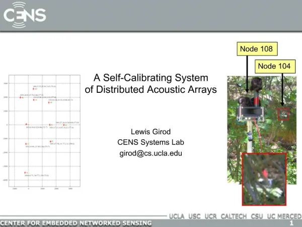
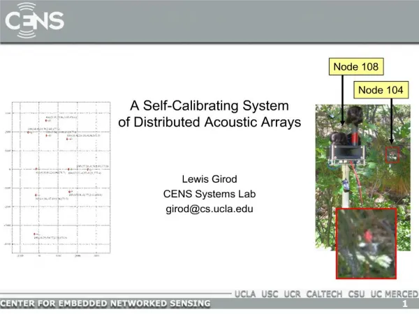
1. 1 A Self-Calibrating Systemof Distributed Acoustic Arrays Lewis Girod
CENS Systems Lab
girod@cs.ucla.edu
2. 2
3. 3 Problem Statement Target System:
Input: Node placement:
3D, Outdoor, Foliage OK
20m Inter-node spacing
Arrays are level
Output: Estimates:
XYZ Position � 25cm
Orientation � 2�
Results in James Reserve
Accurate: Mean 3D Position Error: 20 cm
Precise: Std. Dev. of Node Position: 18 cm
4. 4 Outline Overview of system
Ranging and DOA DSP Algorithm
Performance of Ranging and DOA
Performance of overall system
Conclusions and future work
5. 5 Acoustic Position Estimation System:A Vertical Distributed Sensing Application start by saying vertical application to compute position estiamtes using acoustic ranging etc and this needs all these start by saying vertical application to compute position estiamtes using acoustic ranging etc and this needs all these
6. 6 Position Estimation Application explain pn code ideaexplain pn code idea
7. 7 Acoustic Array Configuration 4 condenser microphones, arranged in a square with one raised
4 piezo �tweeter� emitters pointing outwards
Array mounts on a tripod or stake, wired to CPU box
Coordinate system defines angles relative to array
8. 8 Range and DOA Estimation Inputs:
The input signals from the microphones
The time the signal was emitted (used to select from input signal)
The PN code index used
Outputs
Peak phase (i.e. range)
The 3-D direction of arrival: ?, ?, and a scaling factor V
Signal to Noise Ratio (SNR)
9. 9 Filtering and Correlation Stage Synchronized Sampling Layer completely abstracts application from synchronization details
Correlation
Generate reference signal from PN code index
Correlate against the incoming signal
10. 10 Correlation Signal detection via �matched filter� constructed from PN code
Observed signal S is convolved with the reference signal
Peaks in resulting �correlation function� correspond to arrivals
Earliest peak is most direct path
11. 11 Detection Stage Want to detect first peak above noise floor
Need to capture approx. �peak region� � peak selection refined later
Noise floor is time varying and must be estimated
Use EWMA to compute continuous mean and variance estimate
Selected a such that system adapts to 1% within 5ms
Define threshold to be a multiple of the standard deviation
First value over threshold considered �peak�
How to select threshold?
12. 12 Selecting a Peak Detection Threshold Given a peak detection threshold, e.g. 12, we can determine for any given signal the �noise peak� and �detection peak�.
To be certain not to detect noise, we want a wide gap between the distribution of rejected noise peaks and of detection peaks
We selected a threshold of 12, and tested it with 100,000 trials collected at the James Reserve. picture of noise and detection peaks on this slide with arrows and draw in 12�.picture of noise and detection peaks on this slide with arrows and draw in 12�.
13. 13 Zooming in.. 8x Interpolation Sub-sample phase comparison is critical to DOA estimation
Otherwise, large quantization errors: 1 sample offset = 5�
Once a peak region is identified
Zoom in by interpolating
Use Fourier coefficients to expand the signal at higher resolution
Equivalent to phase shift in FD
But enables direct TD processing of correlation outputs
14. 14 DOA Estimation and Combining Stage 6-way cross-correlation of correlations ? DOA Estimator
Filtered signals from each pair of microphones are correlated
Offset of maximum correlation between pair (�lag�) recorded
DOA Estimator uses least squares to fit �lags� to array geometry
Key: Resilient to perturbations in microphone placement
DOA estimate used to recombine signals to improve SNR
Final peak detection yields range estimate
15. 15 An idea that didn�t work so well: �Angular Correlation� For each possible angle:
Hypothesize incoming angle
Shift correlation functions to match
Multiply and accumulate
Problem:
Too Sensitive to microphone placement
Slight shift misses peaks
16. 16 Position Estimation Problem:
Given pair-wise range and DOA estimates
Estimate X,Y,Z locations and orientation T for each node
Solved using iterative non-linear least squares
17. 17 Experiments Component Testing
Azimuth angle test
Zenith angle test
Range test
18. 18 Experimental Setup for Angular Tests
19. 19 Azimuth Errors as Function of Angle
20. 20 Overall Distribution of Azimuth Errors
21. 21 Zenith Errors as Function of Angle Negative angles are obstructed by the array itself, and have much worse variance.
Zenith performance varies with the azimuth angle, perhaps a function of the array geometry. Our data only tested two azimuth angles.
22. 22 Overall distributions of Zenith Angle The zenith data does not fit well to a normal distribution (which is problematic because the position algorithms assume that).
To improve things slightly, we computed statistics on subsets of the data. Both position algorithms can accept parameterized ? values.
23. 23 Experimental Setup for Range Tests
24. 24 Range Measurements with Mean Error
25. 25 Anomalous Behavior at 50m Might be due to bug in time synchronization service that has since been fixed, or to environmental variables.
26. 26 Overall Distribution of Range Errors Not a particularly good fit to normal distribution
Might improve under more controlled experiment (e.g. lot 4)
Doesn�t account for possible differences node to node
27. 27 System Tests Experimental Process
Lay out 10 nodes, and run system to collect ranges and DOA
Apply positioning algorithms to compute maps
Compare to ground truth
Metrics1
Average Range Residual
Measures quality of fit, useful when GT unknown
Simple average of range residual values
Average Position Error
Absolute measure of performance, useful when GT known
Fit estimated map to ground truth
Then compute average distance between corresponding points
28. 28 Fitting to Ground Truth to get �Fair� Position Error
29. 29 System Test: Court of Sciences 10 nodes placed at yellow dots
Yellow lines denote tall hedges
Ground truth measured as carefully as possible and arrays aligned to point west.
Z axis was difficult to measure; used data from Google Earth, which is measured to the nearest foot.
30. 30 Repeatability: Per-node XY mean and std-dev these show the repeatability of positioning over multiplie experiments
Are non-zero mean due to errors in ground truth or measurementsthese show the repeatability of positioning over multiplie experiments
Are non-zero mean due to errors in ground truth or measurements
31. 31 Z and Orientation mean and std-dev Are non-zero means due to errors in ground truth or in measurements?
X/Y estimates: unclear. Ground truth incorporated cumulative errors and obstructions often blocked efforts to measure both axes.
Z estimates: likely inaccurate. The variation is larger than that expected from Google Earth data.
Orientation estimates: likely accurate: They are generally low-variance and ground truth errors in alignment of 5 degrees are expected.
32. 32 James Reserve System Test Deployed 10 nodes in forested area.
In many cases LOS was partially obstructed.
Ground truth measured using professional surveying equipment.
Nodes were aligned to point approximately west by compass.
33. 33 James Reserve per-node mean and std-dev
34. 34 James Reserve Z and Orientation mean/std-dev For many nodes, the variance in Z values for the hilly JR data is considerably lower than those in the courtyard data.
The orientation repeatability is comparable to the courtyard data.
All data taken from the 6 experiments that placed all 10 nodes. The location stakes are still in place.
35. 35 Conclusions Acoustic ENSbox platform supports distributed acoustic sensing
Implemented ranging and position estimation application.
Highly accurate positioning in a challenging environment
XYZ Position �20cm
Orientation �2�
Nearly order of magnitude improvement upon prior work
9 cm XY error vs. 50 cm (UIUC)
Supports XYZ+T estimation
achieved with
fewer nodes
lower densities
more difficult conditions.
36. 36 Future Work Array geometry calibration, tilt sensor
New tests with better measurement of array orientation
Forward/reverse range discrepancies
Improvements to hardware, array geometry
Development and testing of applications
37. 37 Review of Contributions start by saying vertical application to compute position estiamtes using acoustic ranging etc and this needs all these start by saying vertical application to compute position estiamtes using acoustic ranging etc and this needs all these
38. 38 Thank you!