Download
1 / 5
50 likes | 126 Views
Implementing an advanced framework for CO2 flux analysis using tower and aircraft data, influencing fossil fuel CO2 inventories and functional biosphere responses.

E N D
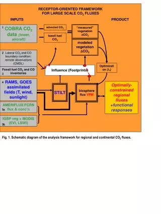
RECEPTOR-ORIENTED FRAMEWORK FOR LARGE SCALE CO2 FLUXES INPUTS PRODUCT advected CO2 COBRA CO2 data (tower, aircraft) 1 “measured” vegetation DCO2 fossil fuel CO2 modeled vegetation DCO2 2 Lateral CO2 and CO boundary condition:remote observations (CMDL) Optimization (i) Influence (Footprints) Fossil fuel CO2 and CO inventories 3 RAMS, GOES assimilated fields (T, wind, sunlight) 4 Optimally-constrained regional fluxes +functional responses biosphere flux VPM STILT AMERIFLUX/FCRN flux & conc’n 5a IGBP veg + MODIS (EVI, LSWI) 5b Fig. 1. Schematic diagram of the analysis framework for regional and continental CO2 fluxes.
Figure 2. (left panels) RAMS mixed-layer hts (Zi) for 1700 UT (1200 EST) for New England and E. Canada, 10 June 2004 (upper) and 11 June 2004 (lower). (middle panels) CO2 concentration cross sections in early morning (upper) and afternoon , 11 June, observed on the red sections of the flight track (right panels). The cross sections followed the movement of the airmass as given by STILT. Note the draw down of CO2 during the day, and the excellent validation of Zi in BRAMS both for the residual layer and the afternoon PBL. 11 June 2004 AM Altitude [km ASL] residual layer PM Altitude [km ASL] Pm PBL Cumulative Distance [km] 11 June 2004 1800UT (1400 EDT) Fig. 3. Observations and environmental forcing from Day 163 (11 June 2004) .(left) B-RAMS PBL mass flux, showing northwesterly flow. (center) GOES-E visible image, showing the cloud field and flow of cool, dry, cloud-free air to Maine. (right, top to bottom) Fig. 4a Fluxes of CO2 at Howland, concentrations at 25 and 100 m at Argyle, and hourly concentration differences at Argyle; flux and gradient reversals are synchronized at 2300-2400 UT, 1-2 hrs before sunset, and likewise 1-2 hours after sunrise. Fig. 4b (left) CO2 land vs sea. (upper) Hourly CO2 (ppm) from Harvard Forest (grey), midday data (black), and 10-day means of midday data (blue); data from Bermuda (orange) and Mauna Loa (red) for comparison. Vertical lines mark the dates for flux reversal. (center) Difference between Harvard Forest midday and Bermuda, color coded by sign of sthe surface flux (emission; uptake). (lower) 24-hr mean tower fluxes mmole m-2s-1). (right, expanded scale)The contrast between surface and overlying CO2 using CMDL aircraft data over Harvard Forest (dashed line, center panel); note that CO2 observed at Bermuda and directly over the tower are very similar. Data sources: Harvard Forest, Barford et al., 2001, updated; Bermuda and aircraft, Tom Conway, CMDL.
Upstream CO2 [ppmv] Forest Observed Cropland Tot Modeled Fossil Fuel Optimized Downstream CO2 [ppmv] 0 (a) Upstream CO [ppbv] Downstream CO [ppbv] (b) CO2 Flux [mmole/m2/s] CO2 Flux [mmole/m2/s] (c) (d) Fig. 5. The framework applied to a Pseudo-Lagrangian experiment over North Dakota (Aug. 2000). Two cross sections were flown at 1400UT and 2100UT on 02 Aug. 2002, about 40 km apart, following the mean air travel. (a) Observed upstream and downstream tracer cross-sections from the ND experiment, showing CO2 and CO. Flight paths are shown in grey. The origin refers to the mean horizontal position of the aircraft during the sampling of the cross-section. The x-axis represents the horizontal location along the first principal component of the aircraft locations. Note the validation of the predicted air flow by tracking the CO maximum in the PBL, which was due to a forest fire plume originating in Canada, and the evident removal of CO2 from the PBL.. (c) The modeled CO2 fluxes attributed to fossil fuel combustion (red dashed), forest (green), and cropland (orange), with Bayesian error estimates. This example sampled mostly cropland (spring wheat). (d) The total constrained biospheric CO2 flux (black dashed)—sum of the separate components in (c), the optimized flux after Bayesian inverse analysis of the GSB (blue dashed), and the observed biospheric flux derived from dividing a simple difference of the vertically integrated CO2 inventories (upstream-downstream, solid black) by the elapsed time [Lin et al. 2004]. The derived fluxes represent the average daytime uptake for CO2 (8 am to 3 pm local standard time). As might have been expected, the uptake magnitude by wheat in North Dakota was notably smaller than the prior (corn, black dashed line) from AmeriFlux.
GOES-8 Visible 8/18/2000 1800 GMT 24h NEE [mmol/(m2 s)] CO2 respiration combust. log10 <<f>>ppm/(mol-m-2s-1) photosynthesis CO Figure 6. Examples of the framework applied to large-scale aircraft data. (upper right) Time integrated footprints from STILT for two continental racetrack patterns flown in COBRA-2003, computed using the EDAS assimilation. There were 176 vertical profiles in 36 flights over 82 hours of flight time. (upper left) Clouds (visible, GOES-8) over eastern N. America on 18 Aug. 2000. (lower) Mean 24-hour NEE for the US using the GSB parameters derived for the northern transect of COBRA-2000 using the framework. Note the strong influence of cloudiness on C exchange fluxes, and the release of CO2 in the drought-affected vegetation of the southern US [from Gerbig et al. 2003b]. Fig. 7. Harvard Forest tower data analyzed using STILT (using the same assimilated meteorological fields that drive the biosphere model) to compute the “influence function” (response [ppm] at the aircraft or tower caused by unit flux at a given time upstream. The optimized GSB flux model from COBRA-2000 was used without adjustment to reconstruct CO and CO2 data observed at Harvard Forest., and to attribute CO2 concentration changes to ecosystem processes (above) and to changing footprint areas (upper left) during the synoptic progression from northerly to westerly flow.
Respiration = αr + (βr× (EVI-EVImin)/(EVImax-EVImin)) Climate data Tower Data Surface Reflectance: MODIS LSWI EVI Validation A priori GPP = (α × Tscalar × Wscalar× Pscalar) × FAPARPAV× PAR Fig. 9. Model (lines) and observed (points) 8-day mean daily GPP (left) and R (right) [units: gC/m2/day], for 2002 at Howland Forest. The model fit optimized 3 parameters in the VPRM (2 for GEE, 1 for respiration, see Fig. 6) for data from 2000-2003, using MODIS time series data (average of 9 1x1 km squares, reported every 8 days) for 9 vegetation types, each with data from eddy tower in the center. These data are tabulated for numerous EOS Land Validation Core Sites (including Harvard and Howland Forests) at http://landval.gsfc.nasa.gov/MODIS/coresite.php. Wscalar= (1 + LSWI)/(1 + LSWImax) ; Pscalar= (1 + LSWI)/2 <budbreak to full canopy; Pscalar= 1 other times> Fig. 8. Schematic of the VPRM [after Xiao et al., 2004] (upper) R in terms of EVI anomaly, giving the spatial variation of biomass with the prior calibrated to flux tower data. (lower ) GPP in terms of FAPAR (=EVI) and LSWI. EVI and LSWI are derived from MODIS data, resolved seasonally and averaged 2003-2004. W accounts for the effect of water stress, and P for phenology. VPRM NEP MODIS EVI gC/m2/d Fig. 10. VPRM example. The VPRM combines data from MODIS (EVI and LSWI, upper left), GOES (lower left), and IGBP (to be replaced by SYNMAP) (lower right) to produce hourly or daily NEP over the study region (upper right) . Results are shown for Maine and S. E. Canada for day 153 (01 June) in 2004. veg. type IGBP GOES shortwave MJ/m2/day


![Using Virtual Tall Tower [CO 2 ] Data in Global Inversions](https://cdn1.slideserve.com/3052018/using-virtual-tall-tower-co-2-data-in-global-inversions-dt.jpg)