Download
1 / 28
290 likes | 487 Views
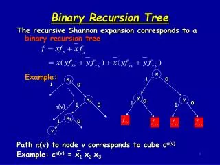
Binary Tree Representation. The recursive Shannon expansion corresponds to a binary tree Example: Each path from the root to a leaf corresponds to a minterm. x. 1. 0. y. y. 1. 0. 0. 1. The root represents the original function f .

E N D
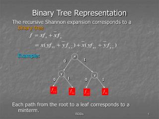
Binary Tree Representation The recursive Shannon expansion corresponds to a binary tree Example: Each path from the root to a leaf corresponds to a minterm. x 1 0 y y 1 0 0 1 BDDs
The root represents the original function f. • The two nodes immediately below the root represent the co-factors of f. • As you go deeper, each node represents a co-factor of the function represented by its parent. • The leaves are the terminal cases representing 0 and 1 which have no co-factors. BDDs
Example Splitting variable a a 1 0 0 1 c b b b 0 1 0 1 0 1 0 1 0 1 0 1 c c 0 1 1 1 0 0 1 0 1 0 BDDs
Implicit Enumeration - Branch and Bound • Checking for tautology and many other theoretically intractable problems (co-NP complete) can be effectively solved using implicit enumeration: • use recursive Shannon expansion to explore Bn. • In (hopefully) large subspaces of Bn, prune the binary recursion tree by • exploiting properties of the node function fc(v) • exploiting heuristic bounding techniques • Even though in the worst case the recursion tree may have 2n nodes, in practice (in many cases), we typically encounter a linear number of nodes. BDDs
Implicit Enumeration - Branch and Bound • Thus we say that the 2n minterms of f have been implicitly enumerated • BDD’s (Binary Decision Diagrams) are alternate representations in which implicit enumeration is performed statically, and nodes with identical path cofactors are identified BDDs
ROBDDs • represents a logic function by a directed acyclic graph (DAG).(many logic functions can be represented compactly - usually better than SOP’s) • canonical form (important) (only canonical if an ordering of the variables is given) • many logic operations can be performed efficiently on BDD’s (usually linear in size of result - tautology and complement are constant time) • size of ROBDD critically dependent on variable ordering BDDs
ROBDDs • one root node per function, two terminals 0, 1 • each node, two children, and a variable • Shannon co-factoring tree, except reduced and ordered(ROBDD) Reduced: • any node with two identical children is removed • two nodes with isomorphic BDD’s are merged Ordered: Co-factoring variables (splitting variables) always follow the same order from a root to a terminal xi1 < xi2 < xi3 < … < xin BDDs
OBDD Ordered BDD (OBDD) Input variables are ordered - each path from root to sink visits nodes with labels (variables) in ascending order. not ordered ordered order = a,c,b a a c c c b b b c 1 1 0 0 BDDs
ROBDD • Reduced Ordered BDD - reduction rules: • if the two children of a node are the same, the node is eliminated: f = cf + c’f • if two nodes have isomorphic graphs, they are replaced by one of them • These two rules added to ordering mean each node represents a distinct logic function. BDDs
F = b’+a’c’ = ab’+a’cb’+a’c’ (all paths to the 1 node) f a 0 1 fa = cb’+c’ c • By tracing paths to the 1 node, we get a cover of pairwise disjoint cubes. • The power of the BDD representation is that it does not explicitly enumerate all paths; rather it represents pathsby a graph whose size is measures by its nodes and not paths. • A DAG can represent an exponential number of paths with a linear number of nodes. 1 fa= b’ b 0 1 0 0 1 BDDs
Examples a a 1 b b c c 0 d d 0 1 0 1 BDDs
EXOR a a b c d = a’b’c’d + a’b’cd’ + a’bc’d’ + ab’c’d’ + a’bcd + ab’cd + abc’d + abcd’ b b c c d d Terms in SOP = ??? Nodes in BDD = ??? 0 1 BDDs
The Ordering Effect root node f = ab+a’c+bc’d a a 1 Two different orderings, same function. c+bd b c c+bd b b 0 c+d d+b d c c c d b b d 0 1 0 1 BDDs
Example f = ad + be + cf There are n! orderings – in this example 6! = 720 Try orderings: a,b,c,d,e,f a,d,b,e,c,f BDDs
Theorem Theorem 1(Bryant – 1986 posted on course page) ROBDD’s are canonical Thus two functions are the same iff their ROBDD’s are equivalent graphs (isomorphic). Of course must use same order for variables. BDDs
Implementation • Each node is a triple (v,g0,g1) representing a function g = v g0 + v g1 • In most implementations, g0 and g1 are pointers to other nodes. BDDs
ITE Operator Table Subset Expression Equivalent Form 0000 0 0 0 0001 AND(f, g) fg ite(f, g, 0) 0010 f > g fg ite(f,g, 0) 0011 f f f 0100 f < g fg ite(f, 0, g) 0101 g g g 0110 XOR(f, g) f g ite(f,g, g) 0111 OR(f, g) f + g ite(f, 1, g) 1000 NOR(f, g) f + g ite(f, 0,g) 1001 XNOR(f, g) f g ite(f, g,g) 1010 NOT(g) g ite(g, 0, 1) 1011 f g f + g ite(f, 1, g) 1100 NOT(f) f ite(f, 0, 1) 1101 f g f + g ite(f, g, 1) 1110 NAND(f, g) fg ite(f, g, 1) 1111 1 1 1 BDDs
Efficient Implementation Strong canonical form: A “unique-id” is associated (through a hash table) uniquely with each element in a set. With BDD’s the set is the set of all logic functions. A BDD node is a function. Thus each function has a unique-id in memory. What is a good hash function? f v 0 1 fv fv BDDs
hash value of key collision chain Unique Table - Hash Table Before a node (v, g, h ) is added to BDD data base, it is looked up in the “unique-table”. If it is there, then existing pointer to node is used to represent the logic function. Otherwise, a new node is added to the unique-table and the new pointer returned. Thus a strong canonical form is maintained. The node for f = (v, g, h ) exists iff(v, g, h ) is in the unique-table. There is only one pointer for (v, g, h ) and that is the address to the unique-table entry. Unique-table allows single multi-rooted DAG to represent all users’ functions: BDDs
Recursive Formulation of ITE v = top-most variable among the three BDD’s f, g, h BDDs
Recursive Formulation of ITE ite(f, g, h) if(terminalcase) { return result; } else if(computed-table has entry (f, g, h )) { return result; } else { let v be the top variable of (f, g, h ); f <- ite(fv , gv , hv ); g <- ite(fv , gv , hv ); if( f equals g ) return g; R <- find_or_add_unique_table(v, f, g ); insert_computed_table( {f, g, h }, R); return R; } } BDDs
Terminal cases: • (0, f, g) = g • (1, f, g) = f • ite (f, g, g) = g • Unique table: Used to ensure one physical representation for any given function. • Computed table: Used to cache results to avoid recomputation. BDDs
Example G H I F a b a a 0 0 0 0 1 1 1 1 D J B C C d b c I = ite (F, G, H) = (a, ite (Fa, Ga , Ha ), ite (Fa , Ga , Ha )) = (a, ite (1, C, H), ite(B,0, H )) = (a, C, (b, ite (Bb , 0b , Hb ), ite (Bb ,0b , Hb)) = (a, C, (b, ite (1,0, 1), ite (0, 0, D))) = (a, C, (b,0, D)) =(a, C, J) b 1 0 1 1 1 0 1 0 1 0 0 D 1 0 0 1 0 1 0 F,G,H,I,J,B,C,D are pointers BDDs
Computed Table Keep a record of (F, G, H ) triplets already computed by the ite operator in a hash-based cache( “cache” table). This means that the collision chain is not used (if collision, old entry thrown away ). The above structure is wasteful since the BDD nodes and collision chain can be merged. BDDs
Edge Complementation G’ G Can combine by making complement edges two different DAGs 0 1 0 1 G G’ only one DAG using complement pointer 0 1 BDDs
V V V V Extension - Complement Edges To maintain the strong canonical form, we need to resolve 4 equivalences: V V V V Solution: Always choose the one on the left, i.e. the “1” edge must not have a complement. BDDs
EXOR (revisited) a a b b b c c c d d d 1 0 1 BDDs