Download
1 / 54
540 likes | 654 Views
This paper discusses advanced methodologies in process modeling utilizing Multivariate Curve Resolution (MCR) techniques, specifically focusing on scenarios with known and unknown reaction mechanisms. It outlines the benefits of using MCR-ALS for analyzing multiset data, including how it overcomes limitations of traditional methods by addressing rank-deficiency and enhancing data robustness. By incorporating various analytic techniques, the study aims to provide a comprehensive understanding of chemical processes and their evolution. The implications of these methodologies for chemical analysis and process monitoring are also explored.

E N D
Advanced process modellingwith multivariate curve resolution Anna de Juan1,(*) and Romà Tauler2. • Chemometrics group. Universitat de Barcelona. Diagonal, 647. 08028 Barcelona. anna.dejuan@ub.edu • Dept. of Environmental Chemistry. IIQAB-CSIC. Barcelona.
Process. Definition and underlying model. • Evolving chemical system monitored by a multivariate signal. • Reaction system with a known mechanism (kinetic process) • Evolving system with inexistent mechanism (chromatographic elution)
= + D DA DB DB DA s s A B c cB A = + c c A B sA sB D s A C ST s B = ST c c A B Bilinear model D = CST + E C D Process. Definition and underlying model.
A B C Time = ST ABC C D Process. Definition and underlying model. Known mechanism Hard-modeling (HM) No mechanism Soft-modeling (SM) Ordered evolving concentration pattern
Process description A B C = Time ABC MCR ST C D 1 0.9 0.8 0.7 2.5 D = CST Concentration 0.6 Absortivities 0.5 2 0.4 0.3 Absorbance 1.5 0.2 0.1 1 Wavelength 0 0 1 2 3 4 5 6 7 8 9 10 Time 0.5 Structural information of compounds (identification) Evolution of process contributions (model) 0 0 10 20 30 40 50 60 70 80 90 100 Wavelength MCR in process analysis Process raw data
Multivariate Curve Resolution – Alternating Least Squares (MCR-ALS) D = CST + E • Determination of the number of components (PCA). • Building of initial estimates (C or ST) (EFA, SIMPLISMA, prior knowledge...) Data exploration Input of external information Iterative least squares calculation of C and ST subject to constraints. Check for satisfactory CST data reproduction. Optimal and chemically meaningful processdescription R. Tauler. Chemom. Intell. Lab. Sys.30 (1995) 133. A. de Juan and R. Tauler. Anal. Chim. Acta500 (2003) 195. J. Jaumot et al. Chemom. Intell. Lab. Sys. 76 (2005) 101.
Constraints Definition Any property systematicallypresentin the profiles of the compounds in our data set. • Chemical origin • Mathematical properties. Application • C and S can be constrained differently. • The profiles within C and ST can be constrained differently. Reflect the inherent order in a process
Unimodality (C) Closure (C) Processes evolving in emergence-decay profiles Mass balance Process constraints Non-negativity (C, S) Selectivity!!
Advantages (low requirements) Bilinear data structure No process model required. No previous identification of process compounds needed. MCR in process modelling Limitations • We model what we measure (non-absorbing species) • Each compound should have a distinct concentration profile and spectrum (rank-deficiency).
Multiset process analysis Incorporation of hard-modelling information MCR in process modelling Limitations • We model what we measure (non-absorbing species) • Each compound should have a distinct concentration profile and spectrum (rank-deficiency).
The same process monitored with different techniques Several processes monitored with several techniques Several processes/batches monitored with the same technique Processes and multiset models
Multiset arrangements. Advantages. • The chemometric reasons • Rotational ambiguity decreases/is suppressed. • Rank-deficiency problems are solved. • Noise effect is minimized • The chemical reasons • More information introduced in the process modelling. • More robustness in the process description. • Better characterization of process compounds (multitechnique analysis). • More global description of process evolution and of effect of inducing agents. (multiexperiment analysis).
ST D C Equally shaped spectra D L (enantiomers) Spectra D = Spectra L Rank 1 Equally shaped concentration profiles A + B C [A] = [B] Rank 2 = Rank-deficient systems(the concept) Detectable rank < nr. of process contributions Rank(D) = min(rank C, rank ST) • Rank-deficiency can be linked to C or to ST
3cA =cB(rank 2) cB cA D1 ST ST D D C C [A]o = 1 [B]o = 3 cA =2cB(rank 2) cB cA D2 [A]o = 2 [B]o = 1 = = Rank-deficient systems(the concept) Equally shaped concentration profiles A + B C Rank 2
3cA =cB cB cA D1 D1 ST ST cA cB = = cB cA D2 D2 cA kcB(rank 3) cA =2cB D D C C [A]o = 1 [B]o = 3 [A]o = 2 [B]o = 1 Rank-deficient systems(the concept)
DUV DUV DCD DCD D D sA sA ksB (rank 2) sB = ST C Breaking rank-deficiency(multiset data) sA = ksB sA ksB sA sA sB sB = SCDT SUVT C
Multitechnique data analysis • Only the concentration direction is shared by all experiments. • Completely different techniques can be treated together • Higher spectral discrimination power among compounds. • The augmented response contains complementary information of all techniques (‘superspectrum’). • The single matrix of process profiles provides cleaner process profiles and a more robust description of the process. • Process profiles are not affected by specific noise patterns of particular techniques. • Process description should be valid for all measurements collected. Multiset multi-way
N N O O Fe Fe pH-induced transitions in hemoglobin Evolution of protein conformations • Global process: many events at different structural levels. • No mechanism defined. • Spectroscopic monitoring between pH 1.5 and 10.5 • Changes in secondary structure UV (350-650 nm), far-UV CD (200-250 nm) • Changes in tertiary structure UV, near-UV CD (250-350 nm), fluorescence (300-450 nm) • Binding of heme group UV, Soret CD (380-430 nm) Muñoz, G.; de Juan, A. Anal. Chim. Acta 2007, 595, 198.
pH-induced transitions in hemoglobin (single technique resolution) 20 20 D2 D1 15 15 10 10 5 5 0 0 -5 -10 -5 -15 -10 380 390 400 410 420 430 200 210 220 230 240 250 0.18 1 0.16 D5 D4 0.14 D2 D3 D4 D5 D1 0.8 0.12 0.1 0.6 0.08 0.4 0.06 0.04 0.2 0.02 0 0 300 350 400 450 350 450 550 650 pH 1.5 10.5 3ary structure Heme binding Global 2ary structure Near-UV CD Soret CD Far-UV CD Fluorescence UV 10 D3 8 6 4 2 0 -2 -4 250 275 300 325 350 Wavelengths (nm) Wavelengths (nm) Wavelengths (nm) Wavelengths (nm) Wavelengths (nm) pH pH pH pH pH
pH-induced transitions in hemoglobin (single technique resolution) • Some chemical events are simpler than the global process. • Non absorbing species are not modelled. • Too similar spectral contributions may not be distinguished. • Multitechnique analysis is needed to complete the puzzle.
Far-UV CD Near-UV CD Soret CD Fluorescence UV 10 D3 8 20 20 D2 D1 15 6 15 10 4 10 5 2 5 0 0 0 -5 -10 -2 -5 Wavelengths (nm) Wavelengths (nm) Wavelengths (nm) Wavelengths (nm) Wavelengths (nm) -15 -4 -10 250 275 300 325 350 380 390 400 410 420 430 200 210 220 230 240 250 0.18 1 0.16 D5 D4 D2 D3 D4 D5 D1 0.14 pH 0.8 0.12 0.1 0.6 0.08 0.4 0.06 0.04 0.2 0.02 0 0 300 350 400 450 350 450 550 650 pH-induced transitions in hemoglobin Global process resolution (multitechnique analysis)
1.2 1 0.8 0.6 0.4 0.2 2 4 6 8 10 pH UV Far-UV CD Fluorescence Near-UV CD Soret CD 0 20 20 20 10 15 10 15 20 5 10 0 10 10 0 5 -10 5 0 0 -5 -20 0 350 400 450 500 550 600 650 250 270 290 310 330 350 195 205 215 225 235 245 300 350 400 450 Wavelengths (nm) Wavelengths (nm) Wavelengths (nm) Wavelengths (nm) Wavelengths (nm) -10 380 390 400 410 420 430 pH-induced transitions in hemoglobin OxyHb D2 D1 Native Hb C Global process resolution S3T(2) S4T(3) S5T(4) S1T(2)* S2T(2) * Figures in parentheses are number of resolved species in single technique analysis. • Non-absorbing species are modelled (Soret CD). • Similar spectral contributions are distinguished (near-UV CD).
Multiexperiment data analysis • Only the spectral direction is shared by all experiments. • No batch synchronisation is needed. • Process induced by different agents and performed in different conditions can be treated together • The single matrix STprovides cleaner pure spectra and a more robust structural characterisationof process compounds. • Easier modelling of minor process contributions by using experiments with complementary information. • Good experimental design may provide experiments with presence/absence of different species. Multiset multi-way
Protein-drug interaction Dominant at low [ligand:protein] ratio and low [ligand]. Protein + TSPP TSPPaggregate [Protein-TSPP]complex Dominant at high [ligand:protein] ratio and high [ligand]. Multiexperiment analysis of experiments enhancing low and high [protein:ligand] ratios help in the definition of all species involved.
7.5 mM 4 0.5 40 m M D2 D1 3.5 0.4 3 2.5 0.3 Absobance (a.u.) Protein concentration TSPP concentration 2 Absorbance (a.u.) 0.2 1.5 1 0.1 0.5 0 0 m 0 M 0 M m 400 500 600 700 400 500 600 700 Wavelength (nm) Protein-drug interaction D1: protein-ligand complex dominates. D2: aggregate dominates
0.35 0.3 0.25 0.2 Absorbance (a.u.) 0.15 ST 0.1 0.05 0 350 400 450 500 550 600 650 700 750 Wavelength (nm) • The different presence/absence of species in D1and D2and the decorrelated information in terms of [TSPP:complex:aggregate] helps to a better definition of the pure spectra. • The aggregate could not be recovered using only D1 • TSPP and the complex are very minor to be correctly recovered only from D2 Protein-drug interaction
Process modelling • Hard-modeling.The variation of a process is fully described by fitting a specific mathematical model (physicochemical or empirical) to the experimental measurements. • Soft-modeling. The variation of a process is described by the bilinear model of the measurements, optimised under chemical and/or mathematical constraints. No explicit mathematical model is used.
D C ST 2.5 1 4 x 10 3 0.9 2 0.8 2.5 0.7 Absorbance 1.5 2 0.6 Concentration Absortivities 0.5 1.5 1 0.4 1 0.3 0.5 0.2 0.5 Non-linear model Fitting min(D(I-CC+) C = f(k1, k2) 0.1 0 0 0 10 20 30 40 50 60 70 80 90 100 0 0 1 2 3 4 5 6 7 8 9 10 0 10 20 30 40 50 60 70 80 90 100 Wavelength Time Wavelengths LS (D, C) (ST) D = CST ;D = CC+D Process hard-modeling • Output:C, S and model parameters. • Unique solutions • The modelmust describeall the experimental variation.
Batch/ exp. 1 ST Batch/ exp. 2 Batch/ exp. 3 = Batch/ exp. n D C Process Hard modeling (multibatch/multiexperiment) Need of one global model or Knowledge of the link expression among different batch models Link among batches model
2.5 4 x 10 3 2 2.5 1.5 2 Absorbance Absortivities 1.5 1 1 0.5 0.5 0 0 10 20 30 40 50 60 70 80 90 100 0 0 10 20 30 40 50 60 70 80 90 100 Wavelength Wavelengths 1 0.9 0.8 0.7 0.6 Concentration 0.5 0.4 0.3 0.2 0.1 0 0 1 2 3 4 5 6 7 8 9 10 Time Soft- modeling (one experiment) ST C D , Constrained ALS optimisation LS (D,C) S* LS (D,S*) C* min (D –C*S*) • Output:C and S. • Solutions might be ambiguous. • All absorbing contributions in and out of the process are modelled.
Batch/ exp. 1 ST Batch/ exp. 2 Batch/ exp. 3 = Batch/ exp. n D C Soft-modeling (multibatch/multiexperiment) Link among batches pure spectra Different experiments can be analysed together Experimental conditions, link among batches may be unknown.
1 1 ABCX ABCX 0.9 0.9 A C A C 0.8 0.8 0.7 0.7 0.6 0.6 Concentration (a.u.) 0.5 0.5 Concentration (a.u.) 0.4 0.4 B B X X 0.3 0.3 0.2 0.2 0.1 0.1 CSM CHM 0 0 0 1 2 3 4 5 6 7 8 9 10 0 1 2 3 4 5 6 7 8 9 10 Time C Time C Non-linear model fitting min(CHM - CSM) CHM = f(k1, k2) Incorporating hard-modeling in MCR • All or some of the concentration profiles can be constrained. • All or some of the batches can be constrained.
ST C D 2.5 1 4 x 10 3 0.9 2 0.8 2.5 0.7 1.5 2 Absorbance 0.6 Concentration Absortivities 0.5 1.5 1 0.4 1 0.3 0.5 0.2 0.5 0.1 0 0 10 20 30 40 50 60 70 80 90 100 0 0 0 1 2 3 4 5 6 7 8 9 10 0 10 20 30 40 50 60 70 80 90 100 Wavelength Time Wavelengths Hybrid hard- and soft-modeling MCR (HS-MCR) • Output:C, S and model parameters. • Hard models and soft-modelingconstraints act simultaneously. • Off-process contributions can be modelled separately. • Process model can be recovered in the presence of absorbinginterferences.
Batch/ exp. 1 ST Batch/ exp. 2 Batch/ exp. 3 = Batch/ exp. n D C HS-MCR (multibatch/multiexperiment) Link among batches (pure spectra) • Global or individualmodels can be used. • Link among different models can be unknown or inexistent. • Model-free and model-based experiments can be analysed together.
Myoglobin denaturation Mechanism Steady-state process Native (N) Intermediate (Is) Denatured (D) Kinetic transient (It) Kinetic process Kinetic process UV spectra, pH-jump stopped-flow First-order consecutive reactions Steady-state process UV spectra, pH range 7.0-2.0 N Is ? D Unknown model P. Culberg, P.J. Gemperline, A. de Juan. (submitted)
. Steady-state unfolding pH pH CpH ST = Kinetic unfolding time time Ct C D Myoglobin denaturation Hard-modelling (kinetic unfolding, 1st order reactions) Soft-modelling constraints Model-free and model-based experiments can be analyzed together.
0 1 Myoglobin denaturation Steady-state process Native (N) Denatured (D) Kinetic transient (It) Kinetic process • Formation of a kinetic transient was detected and hard-modelled. k1 = 4.05 s.1 k2 = 0.62 s-1 • Steady-state unfolding was modelled with soft constraints. time pH Wavelengths
Photodegradation of decabromodiphenil ether Wavelength (nm) Br Br Br O Br Br Br Br Br Br Br BDE-209 (flame retardant) • UV kinetic monitoring in several THF/ water mixtures • (10% water, 20% water, 30% water, 40% water) • Three replicates per solvent composition. S. Mas, A. de Juan, S. Lacorte, R. Tauler (submitted)
Global model 1 One global kinetic model per solvent composition Global model 2 Off-process contribution (spectral solvent effects) k3 k2 k1 D C B A Data arrangement
Photodegradation of BDE-209 k1 k2 k3 D A B C 10% water 20% water 30% water 40% water 2 1 3 2 2 2 1 1 1 3 3 ST C Off-process contribution Rate constants
Low requirements Bilinear data structure No process model required. No previous identification of process compounds needed. High flexibility In data arrangements Multitechnique analysis Multiexperiment analysis. Multitechnique and multiexperiment analysis. In input information Soft-modeling constraints. Hard models. Adaptable to individual compounds and/or experiments. MCR in process modelling. Conclusions
Acknowledgements • Glòria Muñoz (pH-dependent hemoglobin example) • Susana Navea (Protein-drug interaction). • Sílvia Mas (UB and IIQAB-CSIC) (BDE-209 example) • Pat Culberg, East Carolina University (myoglobin example). • Lionel Blanchet, UB and Université des Sciences et Technologies de Lille (photochemical example) • Financial support by Spanish Government • Group Web page: www.ub.es/gesq/mcr/mcr.htm
Process. Definition and underlying model. • Evolving chemical system monitored by a multivariate signal. • Reaction system with a known mechanism (kinetic process) • Evolving system with inexistent mechanism (chromatographic elution) Measurement channel Process variable
2 H 2 H + + CYTOPLASM Q1 Photochemical kinetic process Protein conformational change Fe Q Q Q B i A QH Q Q2 e - 2 Cytochrome 40 Å H Q H A B complex B B 2QH A B 2 P Reaction n center h 4 H + Light on Light off time Protein photochemical reaction Photosynthetic reaction center Rhodobacter Spheroides Measurement: IR rapid-scan spectroscopy (difference spectra) (1200-1800 cm-1) Blanchet, L.; Ruckebusch, C.; Huvenne, J. P.; de Juan, A. Chemom. Intell. Lab. Sys.2007, 89, 26.
Light on time Light off Protein photochemical reaction Q2 P2 = time ST D C Hard-modeling (ubiquinol formation and decay contribution) Soft-modeling constraints Kinetics of ubiquinol are modelled in the presence of an interference (protein absorption).