Download
1 / 62
630 likes | 801 Views
Constraint (Logic) Programming. An overview Optimising Arc Consistency Path Consistency Other forms of consistency Consistency and Constraint Trees [Dech04] Rina Dechter, Constraint Processing,. Maintaining Arc Consistency: From AC-3 to AC-4. Inefficiency of AC-3

E N D
Constraint (Logic) Programming • An overview • Optimising Arc Consistency • Path Consistency • Other forms of consistency • Consistency and Constraint Trees [Dech04] Rina Dechter, Constraint Processing, Foundations of Logic and Constraint Programming
Maintaining Arc Consistency: From AC-3 to AC-4 Inefficiency of AC-3 • Every time a value vi is removed from the domain of some variable Xi, by predicate revise_dom(aij,V,D,C), allarcs leading to that variable are reexamined. • Nevertheless, only some of these arcs aki (for k i and k j ) should be examined. • Although the removal of vi may eliminate one support for some value vk of another variable Xk for which there is a constraint Cki (or Cik), other values in the domain of Xi may maintain support in variable Xifor the pair Xk-vk! • This idea is exploited in algorithm AC-4. Foundations of Logic and Constraint Programming
Maintaining Arc Consistency: AC-4 Algorithm AC-4 (counters): • Algorithm AC-4 maintains data structures to account for the number of values in the domain of variable Xi that support some value vk from another variable Xk, for which there is a constraint Cik. • For example, in the 4 queens problem, the counters that account for the support of value X1= 2 are initialised as follows c(2,X1,X2) = 1 % X2-4 does not attack X1-2 c(2,X1,X3) = 2 % X3-1 and X3-3 do not attack X1-2 c(2,X1,X4) = 3 % X4-1, X4-3 and X4-4 do not attack X1-2 Foundations of Logic and Constraint Programming
sup(2,X1) = [X2-4, X3-1, X3-3, X4-1, X4-3, X4-4] % X1-2 supports (does not attack) X2-4, X3-1, X3-3, ... Maintaining Arc Consistency: AC-4 Algorithm AC-4 (supporting sets) • To update the counters when a value is eliminated, it is useful to maintain the set of Variable-Value pairs that are supported by each value of a variable. • AC-4 thus maintain for each Value-Variable pair the set of all Variable-Value pairs supported by the former pair. sup(1,X1) = [X2-3, X2-4 , X3-2, X3-4, X4-2, X4-3] sup(3,X1) = [X2-1, X3-2 , X3-4, X4-1, X4-2, X4-4] sup(4,X1) = [X2-1, X2-2 , X3-1, X3-3, X4-2, X4-3] Foundations of Logic and Constraint Programming
Maintaining Arc Consistency: AC-4 Algorithm AC-4 (propagation): • Every time that it is detected that a value v from a variable X does not have support in another variable Y, v is removed from the domain of the variable X and is addded to a list for subsequent propagation. • However, although the value may loose support several times, its removal may only be propagated, in a useful way, once. • To account for this situation, AC-4 maintains a Boolean matrix M. The 1/0 value of element M[X,v] represents whether value v is/is not present in the domain of variable X. Foundations of Logic and Constraint Programming
Maintaining Arc Consistency: AC-4 Algorithm AC-4 (Overall Functioning) • AC-4 makes use of the data structures presented in the predictable way. • In a first phase, initialisation, which is executed only once, the algorithm initialises the data structures (counters, supporting sets, boolean matrix and removal list). • In the second phase, propagation, which is executed not only after the first phase, but also after each enumeration step, the algorithm performs the actual constraint propagation, updating the data structures as required. • The two phases are presented next Foundations of Logic and Constraint Programming
AC-4 (Initialisation) procedure initialise_AC-4(V,D,C); M <- 1; sup <- ; List = ; for Cij in Cdo for vi in dom(Xi) do ct <- 0; for vj in dom(Xj) do if satisfies({Xi-vi, Xj-vj}, Cij) then ct <- ct+1; sup(vj,Xj)<-sup(vj,Xj)Xi-vi} end if; end for if ct = 0 then M[Xi,vi] <- 0; List <- List {Xi-vi} dom(Xi) <- dom(Xi)\{vi} else c(vi, Xi, Xj) <- ct; end if end for end for end procedure Foundations of Logic and Constraint Programming
AC-4 (Propagation) procedure propagate_AC-4(V,D,R); while List do List <- List\{Xi-vi} % remove element from List for Xj-vj in sup(vi,Xi) do c(vj,Xj,Xi) <- c(vj,Xj,Xi) – 1 if c(vj,Xj,Xi) = 0 M[Xj,vj] = 1 then List = List {Xj-vj}; M[Xj,vj] <- 0; dom(Xj) <- dom(Xj) \ {vj} end if end for end while end procedure Foundations of Logic and Constraint Programming
Time Complexity of AC-4 Time Complexity of AC-4 (Initialisation): O(ad2). • Analysing the cycles executed in the procedure initialise_AC-4, for Cij in Cdo for vi in dom(Xi) do for vj in dom(Xj) do and assuming that • the number of constraints (arcs) is a, • the variables have all d values in their domains, then the inner cycle of the procedure is executed 2ad2 times, which sets the time complexity of the initialisation phase of AC-4 to O(ad2). Foundations of Logic and Constraint Programming
Time Complexity of AC-4 Time Complexity of AC-4 (Propagation): O(ad2). • In the inner cycle of the propagation procedure a counter for pair Xj-vjis decremented c(vj,Xj,Xi) <- c(vj,Xj,Xi) - 1 • Since there are 2a arcs and each variable has d values in its domain, there are 2ad counters. Each counter is initialised at most to d, as each pair Xj-vj may only have d supporting values in the domain of another variable Xi. • Hence, the inner cycle is executed at most 2ad2 times, which determines the time complexity of the propagation phase of AC-4 to be O(ad2) Foundations of Logic and Constraint Programming
Time Complexity of AC-4 Time Complexity of AC-4 (Overall): O(ad2). • Therefore, the overall time complexity of AC-4 is O(ad2) not only in the beginning (inicialisation + propagation) but also on its subsequent use after each enumeration (propagation alone). • Such assymptotic worst-case complexity is better then that of algorithm AC-3, O(ad3). • Unfortunatelly, this improvement on the time complexity of AC-4 is obtained with a much less favourable space complexity than that of AC-3. Foundations of Logic and Constraint Programming
Space Complexity of AC-4 Space Complexity of AC-4: O(ad2). • As a whole algorithm AC-4 maintains • Counters: As discussed, a total of 2ad • Suporting Sets: In the worst case, for each constraint Rij, each of the d Xi-vi pairs supports d values vj from Xj (and vice-versa). The space to maintain the supporting sets is thus O(ad2). • List: Contains at most 2a arcs • Matrix M: Maintains nd Boolean values. • The space required to maintain the supporting sets dominates. Compared with AC-3, where a space of size O(a)was required to maintain the queue, AC-4 has the much worse space complexity of O(ad2) • Nevertheless, this space complexity is of the same order required to maintain the representation of constraints by extension. Foundations of Logic and Constraint Programming
Is AC-4 optimal? • The assymptotic complexity of AC-4, cannot be improved by any algorithm! • In fact, to check whether a network is arc consistent it is necessary to test, for each constraint Cij, that the d pairs Xi-vi have support in Xj, for which d tests might be required. • Since each of the a constraints must be considered twice, then 2ad2 tests are required, with assymptotic complexity O(ad2) similar to that of AC-4. • However, one should bear in mind that the worst case complexity is assymptotic. For “small” values of the parameters, the constants involved may have a non negligeable effect. • Moreover, in typical cases, most of the data structures used might be unnecessary (or at least optimised). • All things considered, AC-3 outperforms AC-4 almost always, in practice. Foundations of Logic and Constraint Programming
Maintaining Arc Consistency: From AC-4 to AC-6 • Changes to AC-4 - Algorithm AC-6 • Algorithm AC-6 avoids the outlined inefficiency of AC-4 with a basic idea: instead of keeping (counting) all values vi from variable Xi that support a pair Xj-vj, it simply maintains the lowest such vi that supports the pair. • The initialisation of the algorithm becomes “lighter”, since whenever the first value vi is found, no more supporting values are seeked and no counting is required. • AC-6 also does not require the initialisation of supporting sets, i.e. to keep the set of all pairs Xi-vi supported by a pair Xj-vj, but only the lowest such supported vi. • Of course, if these values are not initialised, they must be determined during the propagation phase! Foundations of Logic and Constraint Programming
Complexity of AC-6 Typical complexity of AC-6 • Algorithm AC-6 has a space complexity of O(ad), between O(a)) of AC-3 and O(ad2) of AC-4. Like in AC-4, the time complexity is O(ad2), which is optimal assymptotically. • The worst case time complexity that can be inferred from the algorithms do not give a precise idea of their average behaviour in typical situations. • For such study, one usually tests the algorithms in a set of “benchmarks”, i.e. problems that are supposedly representative of everyday situations. • For these algorithms, either the benchmarks are instances of well known problems (e.g. N-queens), or one relies on randomly generated instances parameterised by • their size (number of variables and cardinality of the domains) ; and • their difficulty (density and tightness of the constraint network). Foundations of Logic and Constraint Programming
16000 14000 12000 10000 # tests and operations AC-3 8000 AC-4 6000 AC-6 4000 2000 0 4 5 6 7 8 9 10 11 Complexity of AC-6 Typical Complexity of algorithms AC-3, AC-4 e AC-6 (N-queens) Foundations of Logic and Constraint Programming
Complexity of AC-6 Typical Complexity of algorithms AC-3, AC-4 and AC-6 (randomly generated problems with variable tightness) n = 12 variables, d= 16 values, density = 50% Foundations of Logic and Constraint Programming
Maintaining Arc Consistency: AC-3d • Bidirectionality of support was also exploited in an adaptation, of both algorithms AC-6 and AC-3, resulting in algorithms A-7 and A-3d. • The main difference between algorithms AC-3 and AC-3d consists of the fact that whenever arc aij is removed from queue Q, the arc aji is also removed, in case it is there. • In this case, both domains of Xi and Xj are revised, which avoids much duplicated work. • Although it does not improve the worst-case complexity of AC-3, the typical complexity of AC-3d seems quite interesting (namely in some problems for which extensive tests were performed). Foundations of Logic and Constraint Programming
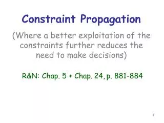
Maintaining Arc Consistency: AC-3d Comparison of Typical Complexity (# of checks) (previous ramdomly generated problems) Foundations of Logic and Constraint Programming
Maintaining Arc Consistency: AC-3d Comparison of Typical Complexity (previous ramdomly generated problems) (equivalent CPU time, in ms, in a Pentium at 200 MHz) Foundations of Logic and Constraint Programming
Maintaining Arc Consistency: AC-3d Comparison of Typical Complexity (previous ramdomly generated problems) (equivalent CPU time, in ms, in a Pentium at 200 MHz) Foundations of Logic and Constraint Programming
Maintaining Arc Consistency: AC-3d • Results seem particularly interesting for problems in which AC-7 was proved much superior to AC-6, both in number of tests and in CPU time. • This is the case of problem RLFAP (Radio Link Frequency Assignment Problem)- • This problem consists of assigning radio frequencies in a safe way (no risk of scrambling), for which instances with 3, 5, 8 e 11 antenae were studied. • The code ( as well as that of other benchmark problems) may be found in a benchmark archive, available from the internet, in URL • http://ftp.cs.unh.edu/pub/csp/archive/code/benchmarks • Together with many other problems, it composes the benchmark web library http://www.csplib.org Foundations of Logic and Constraint Programming
Maintaining Arc Consistency: AC-3d Comparison of Typical Complexity (# of checks) (RFLAP problems) Foundations of Logic and Constraint Programming
Maintaining Arc Consistency: AC-3d Comparison of Typical Complexity (RFLAP problems) (equivalent CPU time, in ms, in a Pentium at 200 MHz) Foundations of Logic and Constraint Programming
Path Consistency • In addition to arc consistency, other types of consistency may be defined for binary constraint networks. • Path consistency is a “classical” type of consistency, stronger than arc consistency, and requiring some “more global view” of the problem, not centered in each constraint in isolation. • The basic idea of path consistency is that, in addition to check support in the arcs of the constraint network between variables Xi and Xj, further support must be checked in the variables Xk1, Xk2... Xkm that form a path between Xi and Xj, i.e. whenever there are constraints Ci,k1, Ck1,k2, ..., Ckm-1, kmand Ckm,j. • In fact, it is possible to show this is equivalent to seek support in any variable Xk,connected to both Xi and Xj. Foundations of Logic and Constraint Programming
Path Consistency Definition (Path Consistency): • A constraint satisfaction problem is path-consistent if, • It is arc-consistent; and • For every pair of variables Xi and Xj, and paths Xi-Xi1- ... - Xik–Xj, the direct constraint Ci,j is tighter than the composition of the constraints in the path Ci,i1, Ci1,i2, ... , Cin,j. • In practice, every value vi in variable Xi must have support, not only in some value vjfrom variable Xj but also in values vi1, vi2 , ... , vin from the domain of the variables in the path. Foundations of Logic and Constraint Programming
Path Consistency • Maintaining this type of consistency has naturally a higher computational cost than maintaining a simpler criterion such as arc consistency. • In order to do so, it is convenient to maintain a representation by extension of the binary constraints, in the form of a boolean matrix. • Assuming that variables Xi and Xj have, respectively, diand djvalues in their domain, constraint Cij is maintained as a boolean matrix Mij of size di*dj. • The value 1/0 of element Mij[k,l] indicates whether the pair {Xi-vk, Xj-vl} satisfies/or not constraint Cij. Foundations of Logic and Constraint Programming
M13[1,2] = M13[2,1]= 1 M13[2,4] = M13[4,2]= 0 Path Consistency Example: 4 queens Boolean Matrix M12, regarding constraint C12 between variables X1 e X2 (or any variables in consecutive rows) M12[1,3] = M12[3,1]= 1 M12[3,4] = M12[4,3]= 0 Boolean Matrix M13, regarding constraint C12 between variables X1 and X2 (or any variables rows separed by one row) Foundations of Logic and Constraint Programming
Checking Path Consistency Checking Path Consistency • To eliminate from matrix Mij (i.e. to zero an element) those values that do not satisfy path consistency through a third variable, Xk, one may use operations similar to matrix multiplication and sum. MIJ <- MIJ MIK MKJ where the operation operates like in a matrix “sum”, but with arithmetic addition replaced by boolean conjunction, and the operation corresponds to matrix multiplication in which arithmetic multiplication and addition are replaced by boolean conjunction and disjunction. • One must still consider the diagonal matrix Mkk to represent the domain of variable Xk. Foundations of Logic and Constraint Programming
Path Consistency: 4 Queens Example (4 queens): • Checking if compound label {X1-1, X3-4} is path inconsistent, through X2. M13[1,4] <- M13[1,4] M12[1,X] M23[X,4] • In fact, M12[1,X] M23[X,4] = 0 since M12[1,1] M23[1,4] % X2-1 does not support {X1-1,X3-4} M12[1,2] M23[2,4] % X2-2 does not support {X1-1,X3-4} M12[1,3] M23[3,4] % X2-3 does not support {X1-1,X3-4} M12[1,4] M23[4,4] % X2-4 does not support {X1-1,X3-4} Foundations of Logic and Constraint Programming
Path Consistency: 4 Queens • Path consistency is stronger than arc consistency, in the sense that its maintenace will allow, in general, to eliminate more redundant values from the domains of the variables than simpler arc consistency is able to do • In particular, for the 4 queens problem, the maintenance of path consistency performs the elimination from the domain of the variables of all the redundant values, that do not belong to any solution, even before any enumeration takes place! • The problem reduced by path consistency may thus be solved with a backtracking-free enumeration. • Notice, that the enumeration and its backtracking is the cause of the exponential complexity of solving non trivial problems. Foundations of Logic and Constraint Programming
Path Consistency: 4 Queens Path consistency in the 4 queens problem Foundations of Logic and Constraint Programming
Path Consistency: 4 Queens Foundations of Logic and Constraint Programming
Maintaining Path Consistency • Of course, this increase in the pruning power of path consistency does not come for free. The computational complexity of achieving and maintaining it is (much) greater than the costs associated with arc consistency. • The algorithms to maintain path consistency, PC-x, have therefore higher complexity than those of the AC-y family. • As an example, algorithm PC-1 (quite simple, with no optimisatiosn) is presented. • The more sophisticated algorithms, PC-2 and PC-4, include optimisations that avoid repetition of tests, much in the same way that the higher members of the AC-y family do. We will simply outline the optimisations and present their complexity. Foundations of Logic and Constraint Programming
Maintaining Path Consistency: PC-1 Algorithm PC-1 procedure PC-1(V,D,C); n <- #Z; Mn <- C; repeat M0 <- Mn; for k from 1 to n do for i from 1 to n do for j from 1 to n do Mijk <- Mijk-1 Mikk-1 Mkkk-1 Mkjk-1 end for end for end for until Mn = M0 C <- Mn end procedure Foundations of Logic and Constraint Programming
Maintaining Path Consistency: PC-1 • Algorithm PC-1: Time Complexity • The main procedure performs a cycle repeat ... until Rn = R0 When there are n2 constraints Cij (dense graph), since each of the corresponding matrix has d2 elements, in the worst case only one element is zero-ed in each cycle. Hence, the cycle can be executed up to n2d2 times. • In each cycle, we have n3 nested cycles of the form for k from 1 to n do for i from 1 to n do for j from 1 to n do Foundations of Logic and Constraint Programming
Maintaining Path Consistency: PC-1 Algorithm PC-1: Time Complexity (cont.) • Each operation Mijk <- Mijk-1 Mikk-1 Mkkk-1 Mkjk-1 requires O(d3) binary operations, since each of the d2 elements is computed through d’s (boolean conjunction) and d-1 operations ’s(boolean conjunction) . • Combining all these factors, the time complexity for PC-1 becomes O(n2d2 *n3 * d3) i. e. O(n5d5) much higher than those obtained with AC algorithms (even AC-1, with complexity O(nad3), presents complexity O(n3d3) for dense networks, for which a n2). Foundations of Logic and Constraint Programming
Maintaining Path Consistency: PC-1 Algorithm PC-1: Space Complexity • The space complexity of PC-1 derives from maintenance of • n3 matrices Mijk, for all sets of constraints Cij, and the paths through a different variable Xk. • The size, d2 elements, of each such matrix. • Hence, the space complexity of algorithm PC-1 is O(n3d2) • This complexity, again much higher than in the AC case (AC-4 has complexity O(ad2) O(n2d2)), is due to the explicit representation of the constraints, and the paths, no more data structures being maintained. Foundations of Logic and Constraint Programming
Maintaining Path Consistency: PC-2 Algorithm PC-2: Complexity • This algorithm maintains a list of the paths that have to be reexamined because of the zero-ing of values in the matrices Mij, (the same principle of AC-3) such that only relevant consistency test are subsequently performed. • In contrast with complexity O(n5d5) of PC-1, the time complexity of PC-2 is O(n3d5) • The space complexity is also better than with PC-1, O(n3d2). For PC-2 the space complexity is O(n3+n2d2) Foundations of Logic and Constraint Programming
Maintaining Path Consistency: PC-4 • Algorithm PC-4: Complexity • By analogy with AC-4, algorithm PC-4, maintains a set of counters and pointers to improve the evaluation of the cases where the removal of an element implies the reevaluation of the paths. • In contrast with the time complexity of PC-1, O(n5d5), and that of PC-3, O(n3d5),the time complexity of PC-4 is O(n3d3) • As expected, the space complexity of PC-4 is worse than that of PC-2, O(n3+n2d2), being similar to that of PC-1, i.e. O(n3d2) Foundations of Logic and Constraint Programming
A node consistent network, that is not arc consistent 0 0 K-Consistency • Node, arc and path consistency, are all instances of the more general case of k-consistency. • Informally, a constraint network is k-consistent when for a group of k variables, Xi1,... , Xik the values in each domain have support in those of the other variables, considering this support in a global form. • The following examples shows a classical example of the advantages of keeping a global view on constraints Foundations of Logic and Constraint Programming
An arc consistent network, that is not path consistent 0,1 0,1 0,1 A path-consistent network, that is not 4-consistent 0..2 0..2 0..2 0..2 K-Consistency Foundations of Logic and Constraint Programming
(Strong) k-Consistency • Definition (k-Consistency): • A constraint satisfaction problem (or constraint network) is 1-consistent if the values in the domain of its variables satisfy all the unary constraints. • A network is k-consistent iff all its (k-1)-compound labels (i.e. formed by k-1 pairs X-v) that satisfy the relevant constraints can be extended with some label on any other variable, to form some k-compound labels that make the network k-1 consistent (satisfy the relevant constraints) . • Definition (Strong k-Consistency): • A constraint problem is strongly k-consistent, if and only if it is i-consistent, for all i 1 .. k. Foundations of Logic and Constraint Programming
A C 0 0 0,1 B (Strong) k-Consistency • A constraint network may be k-consistency but not m-consistent (for m < k). For example, the network below is 3-consistent, but not 2-consistent. Hence it is not strongly 3-consistent. The only 2-compound labels, that satisfy the constraints {A-0,B-1}, {A-0,C-0}, and {B-1, C-0} may be extended to the remaining variable {A-0,B-1,C-0}. However, the 1-compound label {B-0} cannot be extended to variables A or C {A-0,B-0} ! • As can be seen from the definitions, node, arc and path consistency are all instances of strong k-consistency). In fact, a constraint network is • node consistent iff it is strongly 1-consistent. • arc consistent iff it is strongly2-consistent. • path consistent iff it is strongly3-consistent. Foundations of Logic and Constraint Programming
(i,j) -Consistency • The k-consistency criterion may still be extended to a more general criterion of (i,j)-consistency. • A problem is (i,j)-consistent iff all its i-compound labels that satisfy the relevant constraints may be extended with the addition of any j new labels to form a k-compound label (where k=i+j) that still satisfy the relevant constraints . • Of course, k-consistency is equivalent to (k-1,1)-consistency • Although interesting, from a theoretical viewpoint, criteria such as k-consistency and (i,j)-consistency are not maintained in practice (but see algorithm KS-1 [Tsan93]). Foundations of Logic and Constraint Programming
Generalised Arc-Consistency • In the general case of non-binary constraints and constraint networks, the notion of node consistency and its enforcing algorithm NC-1 may be kept, since they only regard unary constraints. • The generalisation of arc consistency for general n-ary constraint networks (for any n > 2) is quite simple. • The concept of an arc must be replaced by that of an hyper-arc, and it must be guaranteed that each value in the domain of a variable must be supported by values in the other variables that share the same hyper-arc (constraint). • Although less intuitive (what is a path in a hyper-graph?), path consistency may still be defined by means of strong 3-consistency for hyper-graphs. Foundations of Logic and Constraint Programming
Maintaining Generalised Arc-Consistency: GAC-3 • In practice, only generalised arc-consistency is maintained, by adaptation of the AC-x algorithms, as is the case of the algorithm GAC-3 below. • To each k-ary constraint one has to consider k directed hyper-arcs to represent the support. procedure GAC-3(V, D, C); NC-1(V,D,C); % node consistency Q={hai..j|Ci..jC...Ci..jC}; %k hyper-arcs while Q do Q = Q \ {hai..j } %removes an element from Q if revise_dom(hai..j,V,D,C) then % Xi revised Q = Q {hak1..kn | Xi vars(Ck2..kn) k1..kn i .. j } end while end procedure Foundations of Logic and Constraint Programming
Maintaining Generalised Arc-Consistency: GAC-3 Algorithm GAC-3: Time Complexity • By comparison with AC-3, predicate revise_dom, checks at most dk(d2) k-tuples of values in k-ary constraints. • Whenever a value vi is removed from the domains of Xi, k-1 hyper-arcs are inserted in queue Q for each k-ary constraint involving that variable. • As a whole, each of the ka hyper-arcs may be inserted (and subsequently removed) (k-1)dtimes from queue Q. All factors considered, the worst case time complexity of algorithm GAC-3 is O(k(k-1)2ad * dk), i.e. O(k2adk+1) • Of course, AC-3, with O(ad3), is the special case of GAC-3 (for k=2). Foundations of Logic and Constraint Programming
Constraint DependentConsistency • The algorithms and consistency criteria considered so far take into no account the semantics of specific constraints, handling them all in a uniform way. • In practice, such approach is not very useful, since important gains may be achieved by using specialised criteria and algorithms. • For example, regardless of more general schemes, it is not useful, for inequality constraints (), when considered separately, to go beyond simple node consistency. • In fact, for Xi Xj, one may only eliminate a value from a variable domain, when the domain of the other is reduced to a singleton. Foundations of Logic and Constraint Programming
Constraint DependentConsistency • Other more specific types of consistency may be used and enforced. For example in the n queens problem, the constraint no_attack(Xi, Xj) • should only be considered when the size of the domain of one of the variables becomes reduced to 3 or less than 3 values. • In fact, if Xi maintains 3 values in the domain, all values in the domain of Xj will have, at least, one supporting value in the domain of Xi. • Thi is because the constraint is simmetrical and any queen may only attack 3 queens in a different row. Foundations of Logic and Constraint Programming