Parallel Computing 2007: Bring your own parallel application
Parallel Computing 2007: Bring your own parallel application. February 26-March 1 2007 Geoffrey Fox Community Grids Laboratory Indiana University 505 N Morton Suite 224 Bloomington IN gcf@indiana.edu. Intel’s Application Stack. Discussed here Rest mainly classic parallel computing.


Parallel Computing 2007: Bring your own parallel application
E N D
Presentation Transcript
Parallel Computing 2007:Bring your own parallel application February 26-March 1 2007 Geoffrey Fox Community Grids Laboratory Indiana University 505 N Morton Suite 224 Bloomington IN gcf@indiana.edu PC07BYOPA gcf@indiana.edu
Intel’s Application Stack Discussed here Rest mainly classic parallel computing PC07BYOPA gcf@indiana.edu
K-Means • The diagrams come from Wikipedia • Take N data points x in some space (can be relatively abstract such as space of chemical properties) • We want to cluster into c components based on distance in space • Algorithm assumes you have a guess ck for cluster centers k=1..c • Associate each of N points with one and only one cluster by minimizing distance to the ck • Replace ck by the centroid of points associated with it • Iterate algorithm PC07BYOPA gcf@indiana.edu
Problem used later in deterministic annealing version of K-Means PC07BYOPA gcf@indiana.edu
K-Meansillustrated a) c) Shows the initial randomized centers and a number of points Now, the association is shown in more detail, once the centroids have been moved. b) d) Centers have been associated with the points and have been moved to the respective centroids Again, the centers are moved to the centroids of the corresponding associated points. PC07BYOPA gcf@indiana.edu
Parallel K-Means • This algorithm is data parallel over N points x • Assign N/Nproc points to each of Nproc processors; no ordering needed in simple algorithm • Broadcast initial cluster centers ck to each processor • Each processor independently calculates nearest ck for each data point it is responsible before • Further it calculates partial sums for c centroids and error estimates (used for convergence) • {Sums over all points} are {Sums over processors (sums over all points in given processor)} • Apply MPI_Allreduce for global sums with (same) c results placed in each processor • All processors calculate new ck and iterate PC07BYOPA gcf@indiana.edu
MPI Parallel Divkmeans clustering of PubChem AVIDD Linux cluster, 5,273,852 structures (Pubchem compound collection, Nov 2005) PC07BYOPA gcf@indiana.edu David Wild Indiana
Performance of Parallel K-Means • There is an an amount of distance calculation that is proportional to (n=N/Nproc)*c for c clusters and N points on Nprocprocessors • There is the global sum calculation proportional to c log2Nproc • So overhead fcomm is log2Nproc tcomm/ntcalc • Appearance of log2Nprocis quite common as global sums over used • That’s why MPI has MPI_Allreduce with hope it can be optimized on whatever network is available • Notice these MPI collectives are often not optimized and rarely used except by Marine Corps • Note this problem has information dimension 1 PC07BYOPA gcf@indiana.edu
Find Maximum of a distributed array TEST • ALLREDUCE can do many reductions typically after user has done reduction internally to each processor PC07BYOPA gcf@indiana.edu
ALLREDUCE on a multicore chip • On a shared memory machine, one can use a different strategy by “transposing” the decomposition so that in global reduction you parallelize over c (the number of) centers not over geometric spatial decomposition • Each core sums over contributions to a given center • Computational Complexity is Max(1, c/Nproc) * Dimension of vector x • Distributed version is c log2Nproc * Dimension of vector x PC07BYOPA gcf@indiana.edu
Transposing Partial Sums Calculate Partial Sums locally 1 2 3 4 C(2,1)C(2,2)C(2,3) C(2,4) C(3,1)C(3,2)C(3,3) C(3,4) C(4,1)C(4,2)C(4,3) C(4,4) C(1,1)+C(2,1)+C(3,1)+C(4,1) C(1,2)+C(2,2)+C(3,2)+C(4,2) C(1,3)+C(2,3)+C(3,3)+C(4,3) C(1,4)+C(2,4)+C(3,4)+C(4,4) 1 2 3 4 C(1,1)C(1,2)C(1,3) C(1,4) Transpose and sum along rows in each processor to get 100% efficiency MPI Solution cannot transpose for free and so uses a tree in this direction • Let result of parallel computation by partial sum C(i,k) for Processor i calculating centroid k • 1≤ i ≤ Nproc and 1 ≤ k ≤ c • Take special case c = Nproc = 4 PC07BYOPA gcf@indiana.edu
Continuing the Intel Homework Set PC07BYOPA gcf@indiana.edu
Clustering by Deterministic Annealing • One can refine this by using multi scale methods and anneal system in position resolution (Gurewitz and Rose) PC07BYOPA gcf@indiana.edu
Deterministically find cluster centers yj using “mean field approximation” – could use slower Monte Carlo PC07BYOPA gcf@indiana.edu
Annealing avoids local minima PC07BYOPA gcf@indiana.edu
Deterministic Annealing • Method does not need to assume a number of clusters • See K. Rose, "Deterministic Annealing for Clustering, Compression, Classification, Regression, and Related Optimization Problems," Proceedings of the IEEE, vol. 80, pp. 2210-2239, November 1998 • Parallelization is similar to ordinary K-Means as we are calculating global sums which are decomposed into local averages and then summed over components calculated in each processor • I found it interesting that clustering (and K-Means) very important in Chemical Informatics for finding related compounds • Field does not seem to know about these multi-resolution methods PC07BYOPA gcf@indiana.edu
Frequent Itemsets Mining • We have a transaction database TDB whose records Tiare a set of items {i1,i2…..im} • The ik are items from a source vocabulary {s1 … sN} and we wish to find frequently occurring itemsets {sA, sB …} based on number of times this itemset appears in any order in a transaction • I looked at two algorithms – Apriori and Frequent Pattern Growth • Apriori focuses on the itemsets searching from smallest to largest systematically • Natural for short transactions and small vocabularies • Frequent Pattern Growth focuses on transactions after re-ordering them in order of item frequency • Superior for finding long itemsets • Effectively generates a new (compact) database with re-ordered items PC07BYOPA gcf@indiana.edu
Parallel Frequent Itemsets Mining • Parallelize by partitioning transaction database and calculating independently frequent patterns from each partition • Use global reduction to accumulate itemset counts from each partition • Now global reduction is summing counts over candidate patterns and goes together with a pruning to only consider patterns with an occurrence > than some threshold • This pruning is not easy to do before global sums (in spite of claims of at least one paper) • The “transposed multicore” ALLREDUCE would be a good strategy PC07BYOPA gcf@indiana.edu
Transposing Partial Itemset Counts Calculate Partial Sums locally 1 2 3 4 C(3,1)C(3,2)C(3,3) C(3,4) C(4,1)C(4,2)C(4,3) C(4,4) C(2,1)C(2,2)C(2,3) C(2,4) C(1,1)+C(2,1)+C(3,1)+C(4,1) C(1,2)+C(2,2)+C(3,2)+C(4,2) C(1,3)+C(2,3)+C(3,3)+C(4,3) C(1,4)+C(2,4)+C(3,4)+C(4,4) 1 2 3 4 C(1,1)C(1,2)C(1,3) C(1,4) Transpose and sum along rows in each processor to get 100% efficiency • Let result of parallel computation by partial sum C(i,k) for Processor i counting occurrences of itemset k • 1≤ i ≤ Nproc and 1 ≤ k ≤ c • Take unrealistic special case c = Nproc = 4 Multicore Algorithm MPI Solution cannot transpose for free and so uses a tree in this direction Distributed MPI_ALLREDUCE PC07BYOPA gcf@indiana.edu
(Mixed) Integer Programming • We are solving an optimization problem such as minimize f(x) = CTx (for linear programming) • Subject to constraints (which are also linear for linear programming) such as AT1x = b1 or AT2x 0 • With constraints that some (mixed case) or all the elements of x are integers (possibly 0 or 1) • The non integer problem is soluble by Simplex method or by interior point methods (Karmarkar) in polynomial time • The integer programming problem is NP complete PC07BYOPA gcf@indiana.edu
Integer Programming Parallelization • Typically one does not parallelize the linear program solver but rather runs this sequentially and instead parallelizes a branch and bound (or cut) search over possible solutions in NP complete case • e.g. search over integer choices for x • The hard integer programming problem consists ofDivide space into subspacesFind upper and lower bounds on f(x) in each subspaceIf lower bound on f(x) in a subspace is greater than current minimum of upper bounds of f(x) in other subspaces (i.e. upper bound of f(x) in any subspace), then one can prune this subspace • If a subspace is still active and upper bound > lower bound, then further divide it into subspaces and iterate process • Parallelism comes from “data parallelism” over subspaces which is suitable for thread based systems • There is typically important shared knowledge such as current minimum upper bound and other information from one subspace that can be re-used by others • Shared (in memory) database for performance PC07BYOPA gcf@indiana.edu
Computer Chess I • Games like computer chess are a special case of the general branch and bound strategy • The space is the set of all moves where N moves by white and black is 2N plys; at each ply there are roughly 35 legal moves so complexity is 352N • Evaluation of of one set of moves to depth 2N is completed by evaluating the final position f(x; x is set of moves) by rules reflecting chess wisdom and summarized by a number (Queen=10, Pawn =1 etc.) • Deep Blue parallelized the calculation of f(x) but here we explore subspace parallelization • We follow work done at Caltech using a 512 node nCUBE which competed as WAYCOOL with poor reliability and results in 1987 and 1988 ACM Computer Chess Championships PC07BYOPA gcf@indiana.edu
Computer Chess II • The upper-lower bound approach is replaced by a minimax principle • Assume f(x) positive is good for white; then at each move white looks at each subspace spawned from the white move and chooses the one with the largest f(x) • In evaluating the subspace we assume that each stage, the side on move makes the best choice • White alwaysmaximizes f(x)at her move and black minimizes f(x) at his move • Of course as N is finite and evaluation function approximate, this is not precise but it gets better and better the larger N is • Note human players tend to use more pattern recognition and less brute force evaluation • Computer games are unimaginative but have fewer errors PC07BYOPA gcf@indiana.edu
Computer Chess III 4 29 13 5 -1 2 15 -7 3 -11 -17 -10 5 • Pruning is illustrated below; as it is advantageous to get (if white is to move) to get a large (good) value of f(x) as early as possible, one sorts moves at each node and looks at the most plausible first • This reduces effective branching ratio from 35 to 6 4 White Maximizes 4 -1 -7 -17 Black Minimizes The dotted lines show subspaces that never need to be searched; this requires that one have done a complete depth search at first subspaces looked at PC07BYOPA gcf@indiana.edu
Computer Chess IV Increasing search depth • Threads were spawned in groups of 4 in Caltech example at different depths of tree and project achieved a speed up of over a 100 and the larger # plys N gets the more parallelism there will be PC07BYOPA gcf@indiana.edu
Computer Chess V • We have subsets of threads (4 in this example) synchronizing on node minimax value • This is a global variable and there are (as in other branch and bound) very important performance gains from a shared position database • This allows scores to be stored for positions and re-used • In chess there are many transpositions leading to identical positions • 1 e4 e5 2 Nf3 Nc6 is identical to (less usual) 1 Nf3 Nc6 2 e4 e5 • There was only a few percent overhead for a distributed database on Caltech distributed memory implementation • Queuing of update requests ensured no errors from multiple threads accessing same location • Multicore architecture should be excellent for this and other large branch and bound and related search algorithms as support shared databases and fast thread synchronization • Note that in Deep Fritz vs. Vladimir Kramnik (human world champion) in November 2006, the program ran on a personal computer containing two Intel Core 2 Duo CPUs, capable of evaluating 8 million positions per second, and searching to an average depth of 17 to 18 ply in the middlegame. Deep Fritz won 4-2 PC07BYOPA gcf@indiana.edu
Wikipedia SVM Example • We are finding optimal hyperplane splitting two samples • Samples are training set • Normal w to splitting hyperplane given byw = i=1n yi i xi • Two samples denoted by crosses yi =1 or circles yi = -1 PC07BYOPA gcf@indiana.edu
Support Vector Machines SVM I • These divide sets by (in simplest case) hyperplanes into two in an optimal least squares fashion • Minimize f() = 0.5 TG - i=1ni • Subject to i=1n yii = 0 and 0 ≤ i ≤ C • With Gij = yiyj K(xi,xj) for Kernel K • This is a training problem where we have a total of n data points from two populations with yi = +1 for first and = -1 for second • K(xi,xj) = xi .xjis simplest case when division is by a hyperplane in space in which x is a vector but Gaussian forms are often usedK = exp(- constant xi-xj2) • G is an n by n dense matrix (n is number of data points) • This is a a quadratic programming QP problem PC07BYOPA gcf@indiana.edu
Support Vector Machines SVM II • Differentiating wrt gives linear equations that must solved iteratively to satisfy inequality constraints • The solver matrix G is both large (106 by 106) and can be dense and this requires large storage space which often exceeds available memory • As in much quadratic programming one can use conjugate gradient solution methods as this identifies systematically the important directions in space (roughly large eigenvalues of positive definite symmetric matrix G) • There are several papers on parallel SVM but I did not see substantial use of parallel implementations • There were two approaches • Either solve the matrix problems in parallel or • Split up dataset and solve multiple subproblems PC07BYOPA gcf@indiana.edu
Support Vector Machines SVM III • Solve the matrix problems in parallel • Interestingly one does not solve full G but iterates up from smaller (~150 by 150) problems and so data parallelism does not exploit size n • Need more reliable SVM solvers for large matrices? • Split up dataset and solve multiple subproblems – Scalable! • Here the difficulty is that essentially you have changed algorithm and it is not clear how best to combine solution of subproblems • But original SVM is full of heuristics (choice of K) so other heuristics may be allowed! • Note whereas multicore appears especially attractive for search problems, it is not so clear for SVM • Multicore does not address huge size of matrix G • High performance matrix solvers are available for distributed memory machines • I suspect there are better “approximate” SVM solvers that will do well on multicore and reduce dimension of G but this is research PC07BYOPA gcf@indiana.edu
Some Parallelization Results from “Parallel Software for Training Large Scale Support Vector Machines on Multiprocessor Systems” This paper reviews much previous work Super linear speedup in (a) due to extra memory PC07BYOPA gcf@indiana.edu