Download
1 / 35
350 likes | 556 Views
Dr. A.K.M. Saiful Islam. Developing ground water level map for Dinajpur district, Bangladesh using geo-statistical analyst. Institute of Water and Flood Management (IWFM) Bangladesh University of Engineering and Technology (BUET). Geo-statistical Analyst of ArcGIS. This training will be on:

E N D
Dr. A.K.M. Saiful Islam Developing ground water level map for Dinajpur district, Bangladeshusing geo-statistical analyst Institute of Water and Flood Management (IWFM) Bangladesh University of Engineering and Technology (BUET)
Geo-statistical Analyst of ArcGIS This training will be on: • Represent data • Explore data • Fit a interpolation Model • Diagnosis output • Create ground water level maps Input Data Groundwater well data of Dinajpur district of Bangladesh
Study Area and Data • Study area • Seven upazillas of Dinajpur District of Bangladesh • Data • Data from 27 Groundwater observation Wells as shape file “gwowell_bwdb.shp”. Weekly data from December to May for 1994 to 2003 • Upazilla shape file “upazila.shp”
Activate Geo-statistical Analyst • Turn on Geostatistaical Anaylst of ArcGIS Enable Extension Enable toolbar
Add Data • Add both shape files
2. Explore Data • Histogram • Normal Q-Q Plot • Trend Analysis • Voronoi Map • Semivariogram • Covariance cloud
a) Histogram • Select attribute: any data e.g. DEC05_1994 • We can change no of bars or bin size • Distribution is normal
Transformation • Log- transformation doesn’t change distribution pattern
b) Normal Q-Q Plot • Normal Q-Q plot is straight line which represents normal distribution
c) Trend Analysis • Shows trend in both X and Y direction since the projection lines (blue and green) are not straight.
d) Voronoi map • Shows the zone of influence of known data points
Shows search directional • Exhibits directional influence in different angle (arrows)
Inverse Distance Weighting (IDW) • Inverse Distance Weighting (IDW) is a quick deterministic interpolator that is exact. There are very few decisions to make regarding model parameters. It can be a good way to take a first look at an interpolated surface. However, there is no assessment of prediction errors, and IDW can produce "bulls eyes" around data locations. There are no assumptions required of the data.
Global Polynomial (GP) • Global Polynomial (GP) is a quick deterministic interpolator that is smooth (inexact). There are very few decisions to make regarding model parameters. It is best used for surfaces that change slowly and gradually. However, there is no assessment of prediction errors and it may be too smooth. Locations at the edge of the data can have a large effect on the surface. There are no assumptions required of the data.
Local Polynomial (LP) • Local Polynomial (LP) is a moderately quick deterministic interpolator that is smooth (inexact). It is more flexible than the global polynomial method, but there are more parameter decisions. There is no assessment of prediction errors. The method provides prediction surfaces that are comparable to kriging with measurement errors. Local polynomial methods do not allow you to investigate the autocorrelation of the data, making it less flexible and more automatic than kriging. There are no assumptions required of the data.
Radial Basis Functions (RBF) • Radial Basis Functions (RBF) are moderately quick deterministic interpolators that are exact. They are much more flexible than IDW, but there are more parameter decisions. There is no assessment of prediction errors. The method provides prediction surfaces that are comparable to the exact form of kriging. Radial Basis Functions do not allow you to investigate the autocorrelation of the data, making it less flexible and more automatic than kriging. Radial Basis Functions make no assumptions about the data.
Kriging • Kriging is a moderately quick interpolator that can be exact or smoothed depending on the measurement error model. It is very flexible and allows you to investigate graphs of spatial autocorrelation. Kriging uses statistical models that allow a variety of map outputs including predictions, prediction standard errors, probability, etc. The flexibility of kriging can require a lot of decision-making. Kriging assumes the data come from a stationary stochastic process, and some methods assume normally-distributed data.
Cokriging • Cokriging is a moderately quick interpolator that can be exact or smoothed depending on the measurement error model. Cokriging uses multiple datasets and is very flexible, allowing you to investigate graphs of cross-correlation and autocorrelation. Cokriging uses statistical models that allow a variety of map outputs including predictions, prediction standard errors, probability, etc. The flexibility of cokriging requires the most decision-making. Cokriging assumes the data come from a stationary stochastic process, and some methods assume normally-distributed data.
Kriging Geo-statistical method • Select ordinary kriging
Semivariogram modeling • Select spherical method
Cross validation • Root mean square error is 1.437
Extent of Map • Set Extend as upazilla
Export as Raster • Select cell size as 100
Zonal statistics • Zonal statistics from Spatial Analyst