Download
1 / 30
300 likes | 477 Views
Robert D. Falgout and Panayot Vassilevski Center for Applied Scientific Computing Lawrence Livermore National Laboratory Germany June, 2003. On Generalizing the AMG Framework. Outline. AMG / AMGe framework background New Measures and Convergence Theory Building Interpolation

E N D
Robert D. Falgout and Panayot VassilevskiCenter for Applied Scientific ComputingLawrence Livermore National LaboratoryGermanyJune, 2003 On Generalizing the AMG Framework
Outline • AMG / AMGe framework background • New Measures and Convergence Theory • Building Interpolation • Compatible Relaxation • Examples • Conclusions and future directions
AMG / AMGe Framework • AMGe heuristic is based on multigrid theory:interpolation must reproduce a mode up to the same accuracy as the size of the associated eigenvalue • Bound a measure (weak approximation property): • Localize the measure to build AMGe components • Several variants developed: E-Free, Spectral • Based on pointwise relaxation • Assumes coarse grid is a subset of fine grid
We are generalizing our AMG framework to address new problem classes • Maxwell and Helmholtz problems have huge near null spaces and require more than pointwise smoothing to achieve optimality in multigrid • Our new theory allows for any type of smoother, and also works for a variety of coarsening approaches (e.g., vertex-based, cell-based, agglomeration) • Paper submitted Model of a section of the Next Linear Collider structure Resonant frequencies in a Helmholtz Application
Preliminaries… • Consider solving the linear system • Consider smoothers of the formwhere we assume that (M+MTA)is SPD (necessary & sufficient condition for convergence) • Note: M may be symmetric or nonsymmetric • Smoother error propagation
Preliminaries continued… • Let P : nc n be interpolation (prolongation) • Let R : n ncbe some “restriction” operator • Note that R is not the MG restriction operator • The form of R will be important later • Define Q : n n to be a projection onto range(P); hence Q=PR such that RP=I
Two new measures • First measure: • Second measure: Defineσ(M) ½(M+MT) , then • Measure is the analogue to the AMGe measure
First measure and MG convergence • Theorem: Assume that the following holds for some constant K:Then, 2-level MG converges uniformly:Here, QA = P(PTAP)-1PTA is the A-orthogonal projector onto range(P) • As in AMGe, we could try to directly localize this new measure to help us build AMG algorithms • But, we will take a different approach
Second measure and MG convergence • Bounding also implies uniform convergence… • Lemma: Assume that (M+MTA) is SPD. Then,where 1 measures the deviation of M from σ(M)and where 0 < max((M)-1A) < 2 . • Must insure “good” constants • in particular, « 2
General notions of C-pts & F-pts • Recall the projection Q=PR, with RP=I • We now fix R so that it does not depend on P • Defines the coarse-grid variables,uc = Ru • Recall that R=[ 0, I ] (PT=[ WT, I ]T) for AMGe; i.e., the coarse-grid variables were a subset of the fine grid • C-pt analogue • Define S : ns n s.t. ns= n nc and RS = 0 • Think of range(S) as the “smoother space”, i.e., the space on which the smoother must be effective • Note that S is not unique • F-pt analogue • S and RT define an orthogonal decomposition of n; any vector e can be written as e = Ses+ RTec
The Min-max Problem • Consider the following base measure, where X is any SPD matrix: • Theorem: Define The arg min satisfies STAP* = 0 and the minimum is • We will call P* the optimal interpolation operator
The Min-max Problem… and AMGe • The optimal interpolation has the general form: • For AMGe, the coarse-grid variables are a subset of the fine grid:Hence,
The Min-max Problem… Spectral AMGe and Smoothed Aggregation (SA) • For Spectral AMGe and SA, the coarse-grid variables are coefficients of basis functions:where the pi are orthonormal eigenvectors of A with eigenvalues 1 … n . Hence, • The optimal interpolation can also be viewed as a “smoothed” tentative prolongator
The new theory separates construction of coarse-grid correction into two parts • The following measures the ability of a given coarse grid c to represent algebraically smooth error: • Theorem: (1) Assume that * K for some constant K.(2) Assume that any one of the following holds for 1:Then, (PR, e) K, e. • (1) insures coarse grid quality –use CR • (2) insures interpolation quality –necessary condition that does not depend on relaxation!
CR is an efficient method for measuring the quality of the set of coarse variables • CR (Brandt, 2000) is a modified relaxation scheme that keeps the coarse-level variables, Ru, invariant • We have defined several variants of CR, and shown that fast converging CR implies a good coarse grid: • Hence, CR can be used as a tool to efficiently measure the quality of a coarse grid! • General idea: If CR is slow to converge, either increase the size of the coarse grid or modify relaxation • F-relaxation is a specific instance of CR
We can use CR to choose the coarse grid • To check convergence of CR, relax on the equationand monitor pointwise convergence to 0 • CR coarsening algorithm:
Using CR to choose the coarse grid • Initialize U-pts • Do CR and redefine U-pts as points slow to converge • Select new C-pts as indep. set over U
Using CR to choose the coarse grid • Initialize U-pts • Do CR and redefine U-pts as points slow to converge • Select new C-pts as indep. set over U
Using CR to choose the coarse grid • Initialize U-pts • Do CR and redefine U-pts as points slow to converge • Select new C-pts as indep. set over U
Using CR to choose the coarse grid • Initialize U-pts • Do CR and redefine U-pts as points slow to converge • Select new C-pts as indep. set over U
Using CR to choose the coarse grid • Initialize U-pts • Do CR and redefine U-pts as points slow to converge • Select new C-pts as indep. set over U
CR based on matrix splittings • Theorem: Assume that (M+MTA) is SPD. Then,where and are as before, and s = ║(I Ms-1As)║As. • Fast converging CR implies good coarse grid • If relaxation is based on a splitting A = M N, then M is explicitly available, and CR is probably feasible
CR based on additive subspace methods • Consider the following additive method:where Ii: ni n and n = irange(Ii). • Define full rank normalized operators Si and RiT s.t. range(Si) = range(IiTS) and range(RiT) = range(IiTRT) • The Ii must be chosen so that Ri Si=0 • Then an additive CR is given by • Same theoretical result as before, but with = 1
CR Additive Schwarz Compatible Additive Schwarz is natural when R=[ 0, I ] • Just remove coarse-grid points from subdomains • It is clear that Ri Si=0 for any choice of Ii Additive Schwarz
More general form of CR • Here, S must be normalized so that STS = I • This variant of CR is always computable • Theoretical result currently requires SPD smoother, M, and involves an additional constant:where [0,1) satisfies
Another general form of CR (due to Brandt and Livne) • As before, S must be normalized so that STS = I • This variant of CR is also always computable • Theoretical result is similar, but weaker:
Anisotropic Diffusion Example • Dirichlet BC’s and (0,1] • Piecewise linear elts on triangles • Standard coarsening, i.e., S = [ I, 0 ]T • The spectrum of the CR iteration matrix satisfies • Linear interpolation satisfies, with = 2,
Anisotropic Diffusion Example – leveraging previous work • Consider the AMGe measure • It is easy to show that ║A║ • As mentioned earlier, this implies • But the AMGe method produces linear interpolation; it is just unable to judge its quality in this setting (i.e., when using line relaxation)
Conclusions and Future Directions • We have developed a more general theoretical framework for AMG methods • Allows for any type of smoother • Allows for a variety of coarsening approaches (e.g., vertex-based, cell-based, agglomeration) • The theory separates construction of coarse-grid correction into two parts: • Insuring the quality of the coarse grid via CR • Insuring the quality of interpolation for the given coarse grid (leverages earlier work) • We have defined several variants of CR • Will explore further the use of CR in practice • Choosing / modifying smoothers automatically?
This work was performed under the auspices of the U.S. Department of Energy by Lawrence Livermore National Laboratory under contract no. W-7405-Eng-48. UCRL-PRES-150807