Advanced Particle-in-Cell Techniques for Plasma Simulation: A Comprehensive Overview
This document offers an in-depth exploration of Particle-in-Cell (PIC) techniques, crucial for simulating plasma phenomena. It discusses the integration of Newton-Lorentz equations with Maxwell's equations, outlining how PIC codes effectively model plasma behavior using representative "super particles." The content covers applications in magnetic fusion, gaseous discharges, and more, alongside the essential coupling between particles and fields. A focus on the Monte Carlo Collision Model (MCC) highlights collision probability and accuracy constraints. This resource is valuable for researchers and educators in plasma physics and computational sciences.

Advanced Particle-in-Cell Techniques for Plasma Simulation: A Comprehensive Overview
E N D
Presentation Transcript
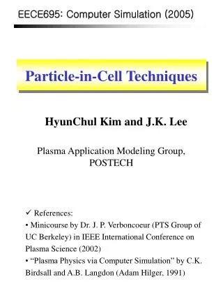
EECE695: Computer Simulation (2005) Particle-in-Cell Techniques HyunChul Kim and J.K. Lee Plasma Application Modeling Group, POSTECH • References: • Minicourse by Dr. J. P. Verboncoeur (PTS Group of UC Berkeley) in IEEE International Conference on Plasma Science (2002) • “Plasma Physics via Computer Simulation” by C.K. Birdsall and A.B. Langdon (Adam Hilger, 1991)
PIC Overview • Applications of PIC model • Basic plasma physics: waves and instabilities • Magnetic fusion • Gaseous discharges • Electron and ion optics • Microwave-beam devices • Plasma-filled microwave-beam devices
PIC Overview • PIC Codes Overview • PIC codes simulate plasma behavior of a large number of charges particles using a few representative “super particles”. • These type of codes solve the Newton-Lorentz equation of motion to move particles in conjunction with Maxwell’s equations (or a subset). • Boundary conditions are applied to the particles and the fields to solve the set of equations. • PIC codes are quite successful in simulating kinetic and nonlinear plasma phenomenon like ECR, stochastic heating, etc.
PIC-MCC Flow Chart • Particles in continuum space • Fields at discrete mesh locations in space • Coupling between particles and fields I II V IV III IV Fig: Flow chart for an explicit PIC-MCC scheme
I. Particle Equations of Motion • Newton-Lorentz equations of motion • In finite difference form, the leapfrog method Fig: Schematic leapfrog integration
I. Particle Equations of Motion • Second order accurate • Requires minimal storage • Requires few operations • Stable for
I. Particle Equations of Motion • Boris algorithm
I. Particle Equations of Motion Finally,
II. Particle Boundary • Absorption • Conductor : absorb charge, add to the global σ • Dielectric : deposit charge, weight q locally to mesh • Reflection • Physical reflection • Specular reflection • 1st order error • Thermionic Emission • Fowler-Nordheim Field Emission • Child’s Law Field Emission • Gauss’s Law Field Emission
II. Particle Boundary • Secondary electron emission + , – – • Photoemission • Ion impact secondary emission • Electron impact secondary emission • Important in processes related to high-power microwave sources
III. Electrostatic Field Model • Possion’s equation • Finite difference form in 1D planar geometry • Boundary condition : External circuit Fig: Schematic one-dimensional bounded plasma with external circuit
III. Electrostatic Field Model From Gauss’s law, • Voltage driven series RLC circuit • From Kirchhoff’s voltage law, • Short circuit • Open circuit
IV. Coupling Fields to Particles • Particle and force weighting : connection between grid and particle quantities • Weighting of charge to grid • Weighting of fields to particles grid point a point charge
IV. Coupling Fields to Particles • Nearest grid point (NGP) weighting • fast, simple bc, noisy • Linear weighting • : particle-in-cell (PIC) or cloud-in-cell (CIC) • relatively fast, simple bc, less noisy • Higher order weighting schemes • slow, complicated bc, low noisy Quadratic spline NGP 1.0 Linear spline Cubic spline 0.5 0.0 Position (x) Fig: Density distribution function of a particle at for various weightings in 1D
IV. Coupling Fields to Particles Areas are assigned to grid points; i.e., area a to grid point A, b to B, etc Fig: Charge assignment for linear weighting in 2D
V. Monte-Carlo Collision Model • The MCC model statistically describes the collision processes, using cross sections for each reaction of interest. • Probability of a collision event • For a pure Monte Carlo method, the timestep is chosen as the time interval between collisions. where 0< R< 1is a uniformly distributed random number. However, this method can only be applied when space charge and self-field effects can be neglected.
V. Monte-Carlo Collision Model • There is a finite probability that the i-th particle will undergo more than one collision in the timestep. Thus, the total number of missed collisions (error in single-event codes) Hence, traditional PIC-MCC codes are constrained by for accuracy.
V. Monte-Carlo Collision Model • Computing the collision probability for each particle each timestep is computationally expensive. • → Null collision method 1. The fraction of particles undergoing a collision each time step is given by 2. The particles undergoing collisions are chosen at random from the particle list. 3. The type of collisions for each particle is determined by choosing a random number, Null collision Collision type 3 Collision type 2 Collision type 1 Fig: Summed collision frequencies for the null collision method.