Download
1 / 32
500 likes | 865 Views
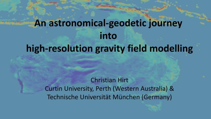
An astronomical-geodetic journey into high-resolution gravity field modelling Christian Hirt Curtin University, Perth (Western Australia) & Technische Universität München (Germany). About the speaker Christian Hirt. 2/30. Education Studies of computer science & geodesy

E N D
An astronomical-geodetic journey into high-resolution gravity field modelling Christian Hirt Curtin University, Perth (Western Australia) & Technische Universität München (Germany)
About the speaker Christian Hirt 2/30 • Education • Studies ofcomputerscience & geodesy • PhD in geodesy (2004) • Positions • Uni Hannover (2001-2006), • Uni Hamburg (2007-2008), • Curtin Uni Perth (since 2009) • Currently • Senior Research Fellow, Curtin University (Perth, Western Australia) & • Hans-Fischer Fellow, Institute forAdvanced Study (Munich, Germany)
3/30 The gravity field of planet Earth • Observations • GPS + Levelling Quasi/geoid heights • Gravimetry Gravity accelerations • Geod. Astronomy Vertical deflections • Torsion Balance Horizontal grav. gradients • … • Models • Regional gravimetric/astro-geoid models (2 km res.) • Geopotential models, e.g., EGM2008 (10 km) • Ultra-high resolution gravity models (GGMplus, 250 m) Geoid „Potdamer Potato“ – view exaggerated
4/30 The gravity field of planet Earth • Observations • GPS + Levelling Quasi/geoidheights • Gravimetry Gravity accelerations 1. Geod. Astronomy Vertical deflections • Torsion Balance Horizontal grav. gradients • … • Models • Regional gravimetric/astro-geoid models (2 km res.) • Geopotential models, e.g., EGM2008 (10 km) • 2. Ultra-high resolution gravity models (GGMplus, 250 m) Geoid „Potdamer Potato“ – view exaggerated
Part 1 Digital Zenith Cameras, vertical deflections and selected results
5/30 Zenith camera – what is this? • Star camera to observe the gravity field • Transportable instrument • Night operation • Delivers vertical deflections (VDs) • Instrumental aspects • Tilt sensors for alignment in plumb line • CCD image sensor for star observation • GPS for timing & geodetic coordinates Hanover Digital Zenith Camera TZK2-D
Geoid Change N 6/30 Zenith camera, GPS and vertical deflections • Determination of the plumb line’s direction and vertical deflections + Digital zenith camera with CCD sensor GPS/GNSS satellite receiver Ellipsoidal normal (,) Plumb line (,) Plumb line (,) Ellipsoidal normal (,) • Vertical deflections (,) • = - = ( - ) cos = cos + sin Vertical Deflection • Vertical deflections important for geodesy (geoid) and geophysics (interpretation) Geoid Ellipsoid
7/30 Geodetic astronomy - from analogue to digital • Analogue era (to the year 2000) • visual or photographic observations • little automation, therefore time-consuming • production of vertical deflections tedious task Comparator for manual star measurement, ETH Zurich • Digital era of geodetic astronomy (J2000) • key feature: CCD (charge-couple-device) image sensor • full automation of observation & image processing • successful developments in Zurich and Hanover • (2001-2003), 10 years in operation Zurich & Hanover digital zenith cameras, operational since 2003
Digital Zenith Cameras State-of-the-art and further developments 8/30 • Example Hanover zenith camera • “One-mouse-click application” – fully automated • ~ 20 min per station incl. data processing • 0.05”- 0.10” accuracy (e.g., Hirt & Seeber 2008, J. Geod) • vertical deflections at ~ 1,000 new stations by now • peak performance of 20 stations per night • Other instrumental developments • Poland (Kudrys 2007), CechRepublic (Ron et al. 2007, 2009), • Serbia (Ogrizovic 2009), USA (NGA, Slater et al. 2009) , • Hungary (Laky 2011), China/Japan (Hanada et al. 2011) • Türkeye (Halicioglu 2012), China (Wang 2013), Hungary (2013) Hanover zenith camera in operation, 2005
Digital Zenith Cameras Some notes on astrometric data processing 9/30 • Image processing • Automated star extraction based on image analysis • Use of point spread functions/centre of mass algorithms • 50 repeat observations ~1000-2000 stars to obtain vertical deflections (2 unknowns) Example of star imagery (0.4 deg2) • Star catalogues • Provide the celestial reference based on Hipparcos (0.001”) • High-accuracy (few 0.01”) and dense catalogues applied to reduce zenith camera star images • e.g., Tycho-2, 2.5 million stars, UCAC-3, 100 million stars ESA’s Hipparcos satellite (1990-1993)
Digital Zenith Cameras Some notes on the accuracy 10/30 • Repeated observations • Station Hannover, 84 nights over 2 years • 24,000 single observations, 225h data • Results • 1 hourobservation: (120 single): 0.05“ • 20 minutesobservation (50 single): 0.08“ • Bywayofcomparion, 0.3“-0.5“ with • analoguecameras, Bürki (1989) • Limiting factor • Anomalousrefraction, externalerror • with 0.01“ to 0.1“ amplitudes Hirt & Seeber 2008, J Geod
Applications for digital astrogeodetic instruments Speaker’s perspective 11/30 • Highly-accurate local geoid determination • mm-quasi/geoid accuracy at local scales (10..50 km) • Validation of gravimetric geoids/ engineering applications • Geophysics Refraction anomaly • Localisation and modelling of mass-density anomalies • Refraction research • Determination and understanding of refraction anomalies Plumb line (,) Ellipsoidal normal (,) • Other applications Mass anomaly • Combined geoid determination (e.g., Austria, Switzerland), • Verification of satellite gravimetry/geopotential models Geoid Ellipsoid
Application example High-resolution local gravity field determination 12/30 • Motivation Observations Minus Mean value Stations Observations • Gravimetric geoid errors increase in mountains • Astrogeodetic method independent and accurate • (mm-accuracy over few 10s of km; Hirt/Flury 2008 JGeod) • Test area and measurements • Isar Valley, Bavarian Alps • 24 km profile, 103 stations (230 m distance) • Profile observed with Hannover digital camera in 2005
13/30 High-resolution local gravity field determination In the Bavarian Alps • Method applied • Astronomical-topographic levelling 1. topographic interpolation of deflections 2. integration of deflections along the profile gives geoid height differences Astrogeodetic geoid profile Isar valley (m) • Comparison with geoid models • German GCG05 geoid: 8 mm RMS (15 mm MAX) • Geoid model of TU Munich (IAPG): • geoid: 4 mm RMS (8 mm MAX) Hirt/Flury 2008 JGeod, Hirt et al. 2007. Differences astrogeoid vs gravimetric geoid (mm)
Vertical deflections in the Bavarian Alps With and without topographic attraction 14/30 Observed vertical deflections (offset subtracted) Mainly show attraction of Topographic masses Topographically reduced (attraction of topography subtracted) Carry geophysical signals
Application example Vertical deflections to validate geopotential models 15/30 Geopotential models From the GOCE satellite mission (100 km resolution) Validation Observed astrogeodetic Vertical deflections EGM2008 – a global geopotential model with 10 km resolution
Application example Vertical deflections (VD) to validate geopotential models 16/30 • Basic problem: spectral differences • VD from observation contain full gravity spectrum Astrogeodetic observation • VD from geopotential models (GOCE, EGM2008) • do not contain short-wavelength signals Spectral resolution Long scales short scales Missing signals Geopotential model Max. spherical-harmonic degree of model, e.g. GOCE: 250, or EGM2008: 2160 • Solutions • Low-pass filtering of observations (e.g., Voigt et al. 2012) • Spectral augmentation of geopotential model (e.g. Hirt 2010 JGeod)
Application example Vertical deflections (VD) to validate geopotential models 17/30 • Spectral augmentation of geopotential models • Use of high-resolution topography models as a data source • High-pass filtering (commensurate with geopotential model) • Forward-modelling of gravitational effects • VD can reach ~20 arc-sec amplitudes @ scales < 10 km in the Mountains • Not represented in EGM2008, but modelled here (Hirt 2010 JGeod)
18/30 Validation of EGM2008 from astrogeodetic vertical deflections • Ground truth data • 1060 astrogeodetic VDs over Europe • From zenith camera observations Harz • Results Swiss Bavaria • EGM2008 reaches 3“ VD accuracy, but Portugal Greece • EGM2008 + Spectral augmentation delivers 1“ VD accuracy over Europe (Hirt et al. 2010 JGR), also over North America and Australia RMS = 1“ RMS = 3“ Withspectralaugmentation Data courtesy: Swiss Geodetic Commission, Drs. Bürki und Marti, Hanover zenith camera observations 2003-2006
19/30 Validation of GOCE geopotential models from astrogeodetic vertical deflections • Principle: GOCE-augmentation with EGM2008 & Topo 1060 European VDs (ground truth) GOCE Missing signals GOCE EGM2008 Topography GOCE Topography EGM2008 GOCE Topography EGM2008 GOCE EGM2008 Topography GOCE EGM2008 Topography Harmonic degree (2..250) 2160 216,000 • Results • new GOCE modelsrepresentgravityfield • wellton=200..220 (100 km scales) • Astrogeodetic VDs are sensitive • toevaluatesatellitegravimetry RMSe of Astro VD minus modeled VD
Part 2 Modelling of Earth‘s gravity field with ultra-high resolution
Gravity modelling with ultra-high resolution 20/30 • Limited resolution of geopotential models • GOCE (satellite gravimetry): degree ~200 (100 km) • EGM2008 (GRACE+terrestrial gravity): degree 2160 (10 km) • But many applications need full-spectrum gravity • E.g., calibration of scales (gravity corrections) • Estabishment of geodetic height systems (gravity corrections) • Topographic heighting with GPS (geoid as a correction) • Forward-modelling to augment geopotential models • Based on digital elevation/mass models • Gives more complete gravity information, e.g., for engineering & geodesy
21/30 Gravity modelling with ultra-high resolution • Augmentation principle can be used to „construct“ • ultra-high resolution gravity maps - locally • Example gravity disturbances over Bavarian Alps 30 km = + 30 km … gives gravity @ 200 m resolution 10 km resolution from EGM2008 10 km – 200 m resolution from SRTM topography
Gravity modelling with ultra-high resolution 22/30 • Can be done regionally Gravity disturbances over Switzerland, unit mGal • And globally …
Global gravity modelling with ultra-high resolution 23/30 • Project: Construction of 200 m resolution gravity maps • World-wide over land areas • Based on newest satellite gravity (GRACE/GOCE) and EGM2008 • SRTM-topography to provide short-scale gravity field • through forward-modelling • Challenge computation time • At 200 m resolution, thereare > 3 billionlandpoints • Forward-modellingis time-consuming (e.g., 5 pts/s) • 20 yearscomputation time (@ 1 CPU) • Parallelisationanduseofsupercomputers • 3 weeks (max. 1100 CPUs) tocomplete
Global gravity modelling with ultra-high resolution – not impossible 24/30 • New global gravity maps GGMplus • GOCE, GRACE, EGM2008 combined • with SRTM topography • near global coverage @ 200 m • first work-of-its-kind • GGMplus provides… GGMplus gravity anomalies at 3 billion land points (Hirt et al. 2013, Geoph. Res. Letters) • Maps of frequently used functionals of the • gravity field (gravity/geoid/vertical deflections) geodesy.curtin.edu.au/GGMplus/ • Freely for science, industry and education
25/30 GGMplus at the place of this presentation Latitude = 47°41′ Longitude =16°36′ • Gravity disturbances & gravity accelerations
GGMplus at the place of this presentation Latitude = 47°41′ Longitude =16°36′ 26/30 • Vertical deflections (without zenith camera!)
GGMplus - a new picture of Earth‘s gravity field at ultra-high resolution 27/30 • New statistics of the gravity field – gravity accelerations Model Minimum (all m/s2) Maximum Peak-to-peak GRS80 field9.7803 (Equator) 9.8322 ( Poles) ~0.05 GGMplus9.7639 (Peru) 9.8337 (near Northpole) ~0.07 . (Hirt et al. 2013, Geoph. Res. Letters) • Where is g likely to be smallest? • Nevado Huascaran summit, Andes, Peru • Candidate location for minimum g-value • Measurements to confirm… Nevado Huascaran, Peru
GGMplus – new continental gravity maps Between ±60° latitude 28/30 All data freely available via geodesy.curtin.edu.au/GGMplus/
GGMplus – Accuracy & Limitations 29/30 • Estimated accuracy of GGMplus Functional Europe/North-America/Australia Asia/Africa/South-America Gravity < 5 mGal ~10-20 mGal Deflections 1 arc-sec ~3-5 arc-sec Geoid < 0.1 m ~ 0.3 m • Whatitcanandcan‘tbeusedfor Geological interpretation at short scales (10 km to 200 m not observation-based) Gravity reference model – GGMplus requested/tested by industry & Western Australian government Gravity corrections (engineering/geodesy)
30/30 Web resources for data and models • Digital zenith camera – technology & outcomes • Hirt., C; Bürki, B.; Somieski, A.; Seeber, G. Modern Determination of vertical deflections using digital zenith cameras. Journal Surveying Engineering 136(1), Feb 2010, 1-12. http://en.wikipedia.org/ wiki/Zenith_camera • Ultra-high resolution gravity maps GGMplus http://geodesy.curtin. edu.au/GGMplus/ complete Hungary @ 200 m resolution